Transcriptional analyses
Source:vignettes/transcriptional_analyses.Rmd
transcriptional_analyses.RmdThis vignette demonstrates how to perform transcriptional analyses using the macpie package, focusing on differential gene expression and pathway enrichment in high-throughput transcriptomic screening datasets. The workflow builds on a tidySeurat object and applies standardised, scalable tools to compare treatment conditions against controls.
Key points:
- use compute_single_de to perform a differential expression analysis for one treatment group vs control
- use compute_multi_de to perform differential expression analyses for all treatment groups vs control
- use volcano plot, box plot and heatmap to show results from the
analyses and visualise gene expression levels
- use enrichr for pathway enrichment analysis
1. Data import
Data access
The full dataset (>10 MB of.rdsfiles) is currently under restricted release and will become publicly available upon publication (at Zenodo).
In the meantime, please contact us for early access.
Data is imported into a tidySeurat object, which allows the usage of both the regular Seurat functions, as well as the functionality of tidyverse.
If the samples are spread across multiple plates, users can submit a vector of directories (or named directories, where names will become barcode prefixes) instead of one directory to the Read10X function.
#install.packages("macpie")  # or devtools::install_github("PMCC-BioinformaticsCore/macpie")


library(macpie)
suppressPackageStartupMessages(
  library(enrichR)
)
library(pheatmap)

# Define project variables
project_name <- "PMMSq033"
project_metadata <- system.file("extdata/PMMSq033_metadata.csv", package = "macpie")
# Load metadata
metadata <- read_metadata(project_metadata)


# 1. Load your own gene counts per sample or 2. data from the publication
project_rawdata <- paste0(dir, "/macpieData/PMMSq033/raw_matrix")

project_name <- "PMMSq033"
raw_counts <- Read10X(data.dir = project_rawdata)

# Create tidySeurat object
mac <- CreateSeuratObject(counts = raw_counts,
                          project = project_name,
                          min.cells = 1,
                          min.features = 1)

# Join with metadata
mac <- mac %>%
  inner_join(metadata, by = c(".cell" = "Barcode"))

# Add unique identifier
mac <- mac %>%
  mutate(combined_id = str_c(Treatment_1, Concentration_1, sep = "_")) %>%
  mutate(combined_id = gsub(" ", "", .data$combined_id))

# Filter by read count per sample group
mac <- filter_genes_by_expression(mac,
                                  group_by = "combined_id",
                                  min_counts = 10,
                                  min_samples = 2)
# Subset the working dataset
mac <- mac %>%
  filter(Project == "Current")
2. Single comparison
Similar to scRNA-seq data, MAC-seq gene expression counts have an excess of zero counts compared to bulk RNA-seq. Statistical models assuming a Poisson or negative binomial distribution may not fit the data distribution well. Additionally, replicates can be quite variable due to a large number of potential latent effect during high-throughput screening, and should be assessed during the QC process.
One way to assess the quality of normalization methods is with the average coefficient of variation across the samples.
# First we will subset the data to look at control, DMSO samples only
mac_dmso <- mac %>%
  filter(Treatment_1 == "DMSO")

# Run the RLE function to compare data normalisations
plot_rle(mac_dmso, label_column = "Row", normalisation = "edgeR")
#> tidyseurat says: Key columns are missing. A data frame is returned for independent data analysis.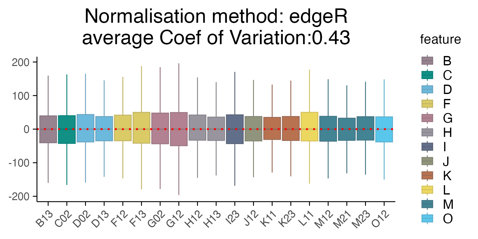
plot_rle(mac_dmso, label_column = "Row", normalisation = "limma_voom")
#> tidyseurat says: Key columns are missing. A data frame is returned for independent data analysis.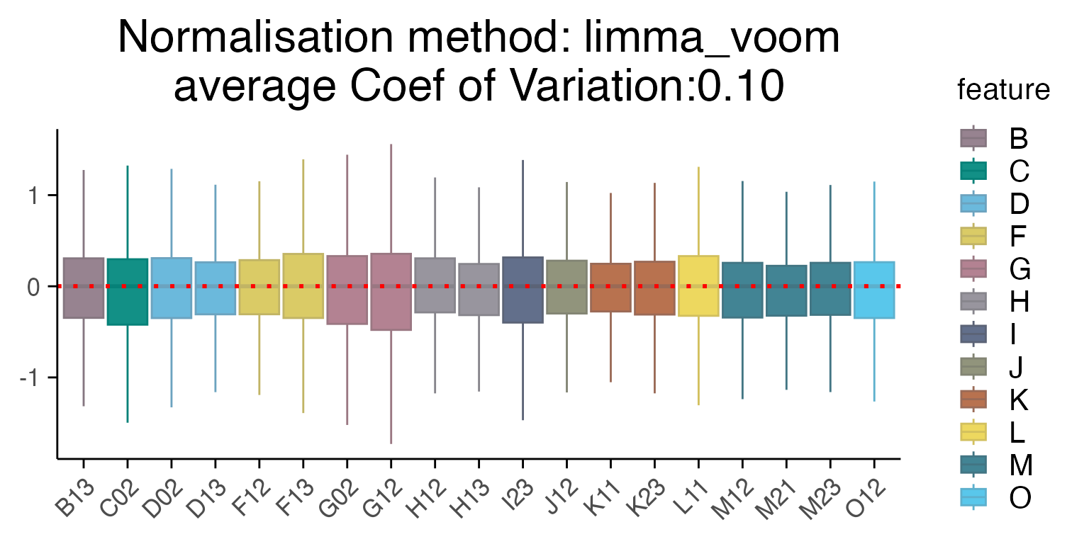
# For multiple plates, once can add a vector with batch factors, for example
# plot_rle(mac_dmso, label_column = "Row", normalisation = "limma_voom", batch = mac_dmso$Plate_ID)
Normalised data for evaluation of normalizations with other methods (such as plotMA etc) can be extracted with:
normalised_counts <- compute_normalised_counts(mac_dmso, method = "SCT", 1)Similarly, influence of DE methods on volcano plots can be easily assessed.
# First perform the differential expression analysis
treatment_samples <- "Staurosporine_10"
control_samples <- "DMSO_0"
top_table <- compute_single_de(mac, treatment_samples, control_samples, method = "limma_voom")

top_table_2 <- compute_single_de(mac, treatment_samples, control_samples, method = "edgeR")
# Let's visualise the results with a volcano plot
p1 <- plot_volcano(top_table, max.overlaps = 18) + ggtitle("limma_voom")
p2 <- plot_volcano(top_table_2, max.overlaps = 18) + ggtitle("edgeR")
p1+p2
#> Warning: ggrepel: 853 unlabeled data points (too many overlaps). Consider
#> increasing max.overlaps
#> Warning: ggrepel: 384 unlabeled data points (too many overlaps). Consider
#> increasing max.overlaps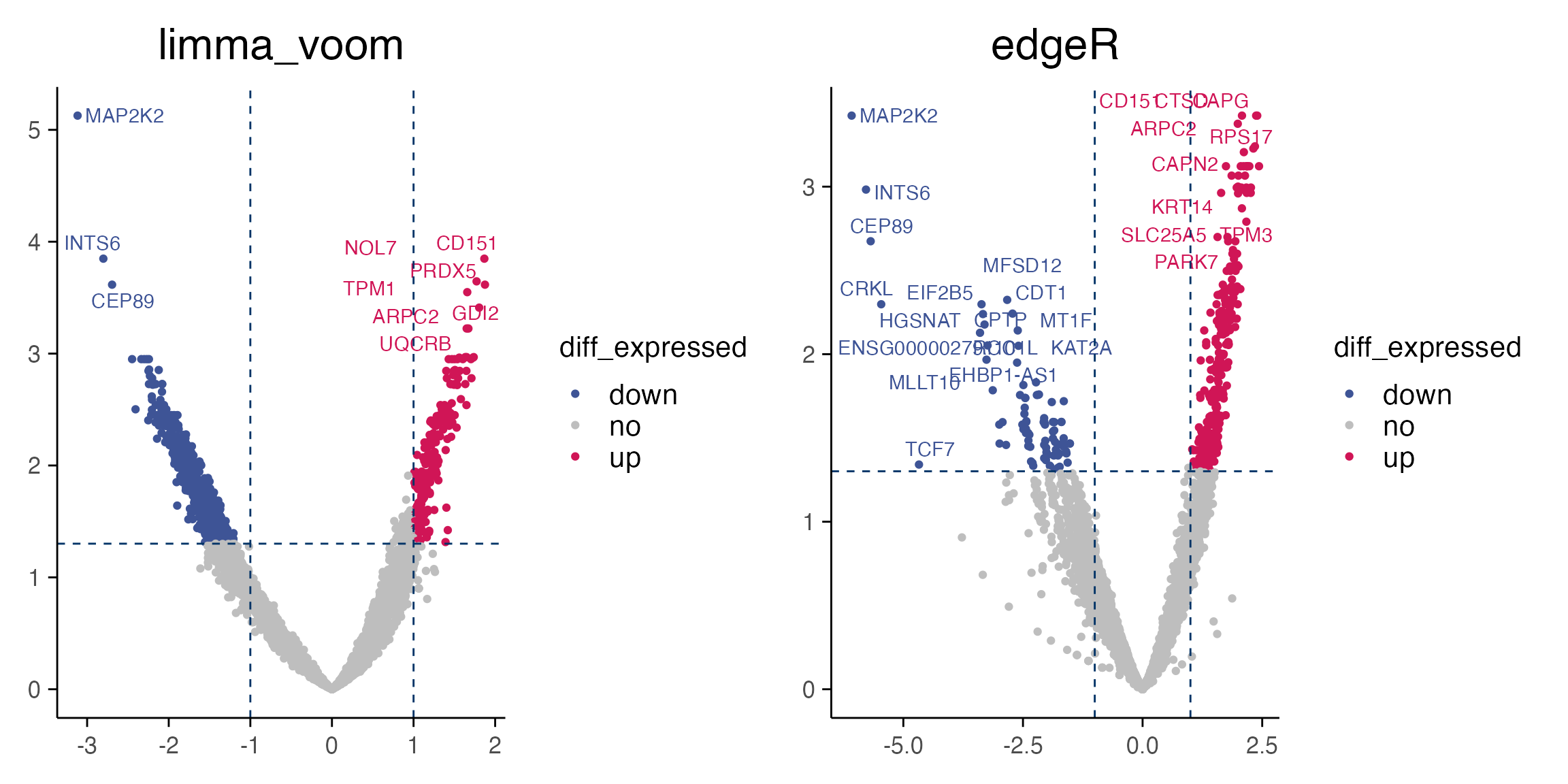
Based on the results, we can quickly check gene expression levels in counts per million (CPM) for selected genes between treatment and control samples as described below.
genes <- top_table$gene[1:6]
group_by <- "combined_id"
plot_counts(mac,genes, group_by, treatment_samples, control_samples, normalisation = "cpm", color_by = "combined_id")
#> Normalizing layer: counts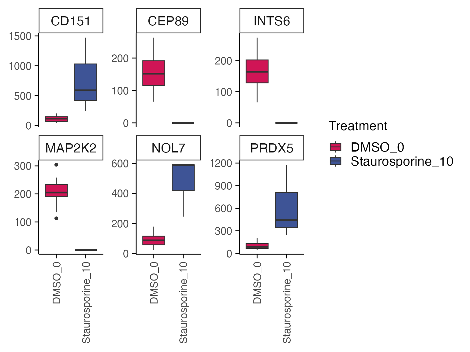
Some plotting functions also have a “summarise” version that provides collapsed versions of the results in a table format.
print(summarise_de(top_table, lfc_threshold = 1, padj_threshold = 0.01), width = Inf)
#> # A tibble: 1 × 6
#>   Total_genes_tested Significantly_upregulated Significantly_downregulated
#>                <int>                     <int>                       <int>
#> 1               5660                       128                         234
#>   Total_significant Padj_threshold Log2FC_threshold
#>               <int>          <dbl>            <dbl>
#> 1               362           0.01                1
3.2. Pathway analysis
Differential gene expression results for individual comparisons of treatment vs control in macpie are performed with enrichR, which has access to a number of curated gene sets available through enrichR::listEnrichrDbs(). In the following case, the effect of Staurosporine on breast cancer cells through Myc inactivation can be observed through pathway enrichment analyses.
top_genes <- top_table %>%
  filter(p_value_adj < 0.01) %>%
  select(gene) %>%
  pull()

enriched <- enrichR::enrichr(top_genes, c("MSigDB_Hallmark_2020","DisGeNET",
                                 "RNA-Seq_Disease_Gene_and_Drug_Signatures_from_GEO"))
#> Uploading data to Enrichr... Done.
#>   Querying MSigDB_Hallmark_2020... Done.
#>   Querying DisGeNET... Done.
#>   Querying RNA-Seq_Disease_Gene_and_Drug_Signatures_from_GEO... Done.
#> Parsing results... Done.
p1 <- enrichR::plotEnrich(enriched[[1]]) +
  macpie_theme(legend_position_ = 'right') +
  scale_fill_gradientn(colors = macpie_colours$divergent)
#> Scale for fill is already present.
#> Adding another scale for fill, which will replace the existing scale.

gridExtra::grid.arrange(p1, ncol = 1)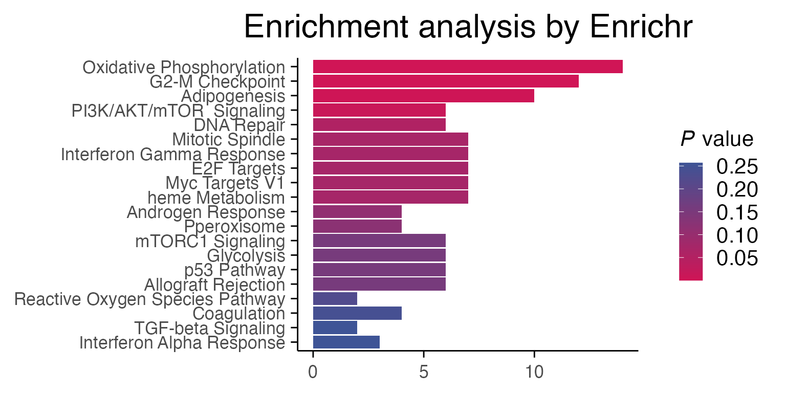
While using “MSigDB_Hallmark_2020” is a standard, if you check the data from “DisGeNET”, you will see that our MCF7 (breast cancer cell line) samples are correctly enriched for breast cancer profiles.
p1 <- enrichR::plotEnrich(enriched[[2]]) +
  macpie_theme(legend_position_ = 'right') +
  scale_fill_gradientn(colors = macpie_colours$divergent)
#> Scale for fill is already present.
#> Adding another scale for fill, which will replace the existing scale.
gridExtra::grid.arrange(p1, ncol = 1)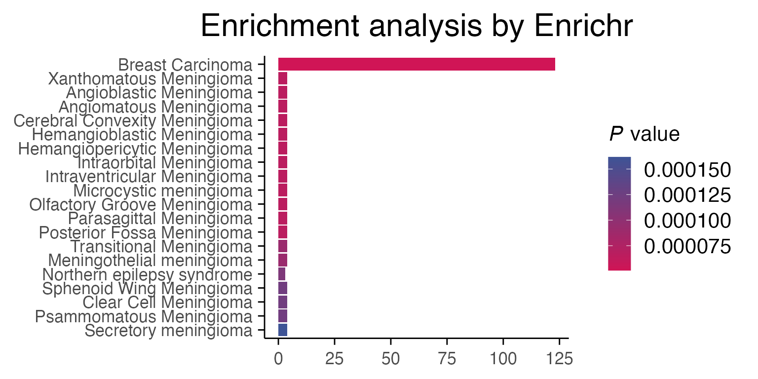
3.3. Differential gene expression - multiple comparisons
Since MAC-seq is commonly used for high-throughput screening of compound libraries, we often want to compare multiple samples in a screen vs the control. This process can easily be parallelised. First we select a vector of “treatments” as combined_ids that do not contain the word “DMSO”. (Warning, due to the limitations of “mclapply”, parallelisation speedup currently only works on OSX and Linux machines, and not on Windows.)
mac$combined_id <- make.names(mac$combined_id)

treatments <- mac %>%
  filter(Concentration_1 == 10) %>%
  select(combined_id) %>%
  filter(!grepl("DMSO", combined_id)) %>%
  pull() %>%
  unique()
#> tidyseurat says: Key columns are missing. A data frame is returned for independent data analysis.
mac <- compute_multi_de(mac, treatments, control_samples = "DMSO_0", method = "limma_voom", num_cores = 1)
If we want to see how individual genes are expressed across the treatment groups, we can use two approaches. First, we can visualise expression of a specific list of genes on a heatmap.
plot_multi_de(mac, group_by = "combined_id", value = "log2FC", p_value_cutoff = 0.01, direction="up", control = "DMSO_0", by="fc", gene_list = head(top_genes, 10))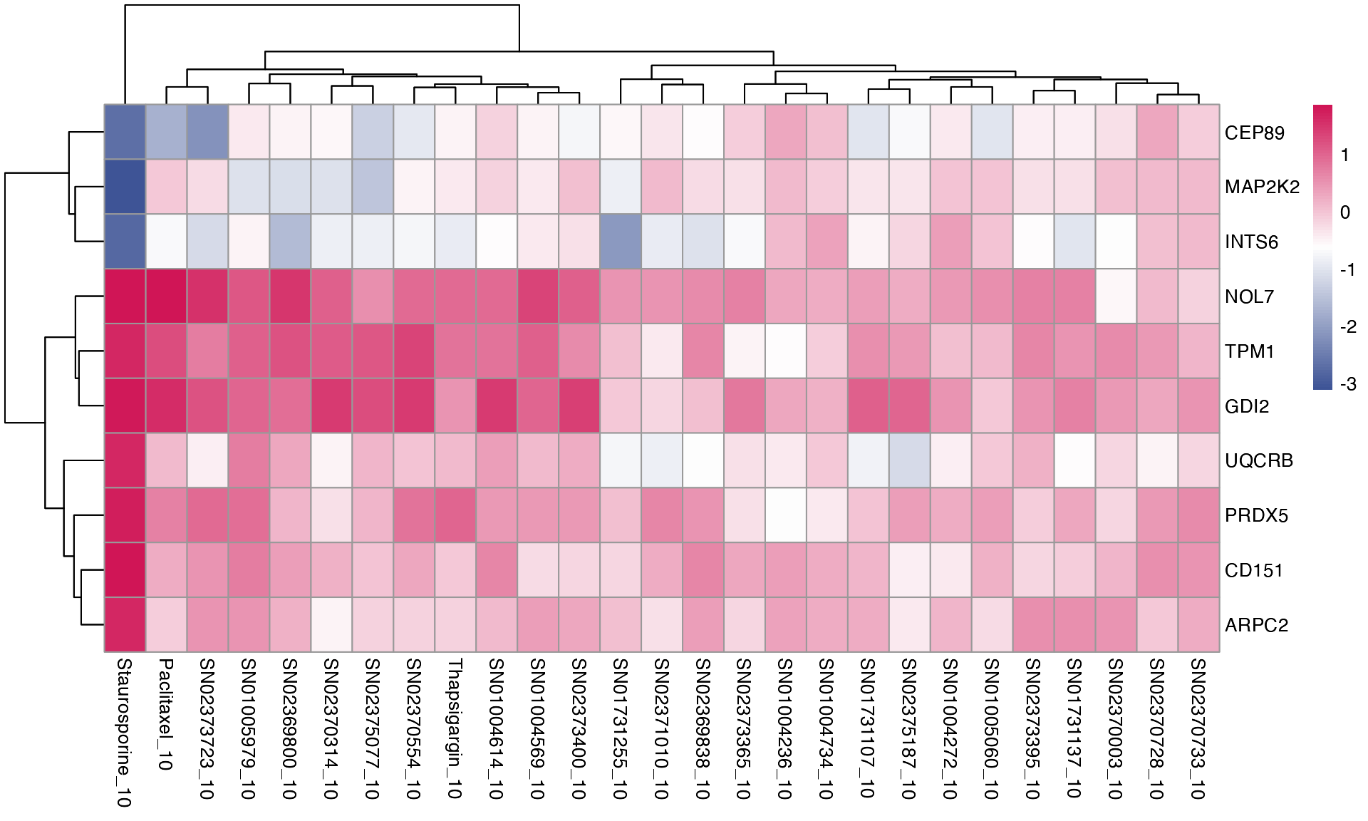
Second, we can visualise shared differentially expressed (DE) genes, defined as the top 5 DE genes from each single drug comparison (treatment vs control) that are found in at least 2 different treatment groups. The heatmap below represents log2FC values of DE genes.
plot_multi_de(mac, group_by = "combined_id", value = "log2FC", p_value_cutoff = 0.01, direction="up", n_genes = 5, control = "DMSO_0", by="fc")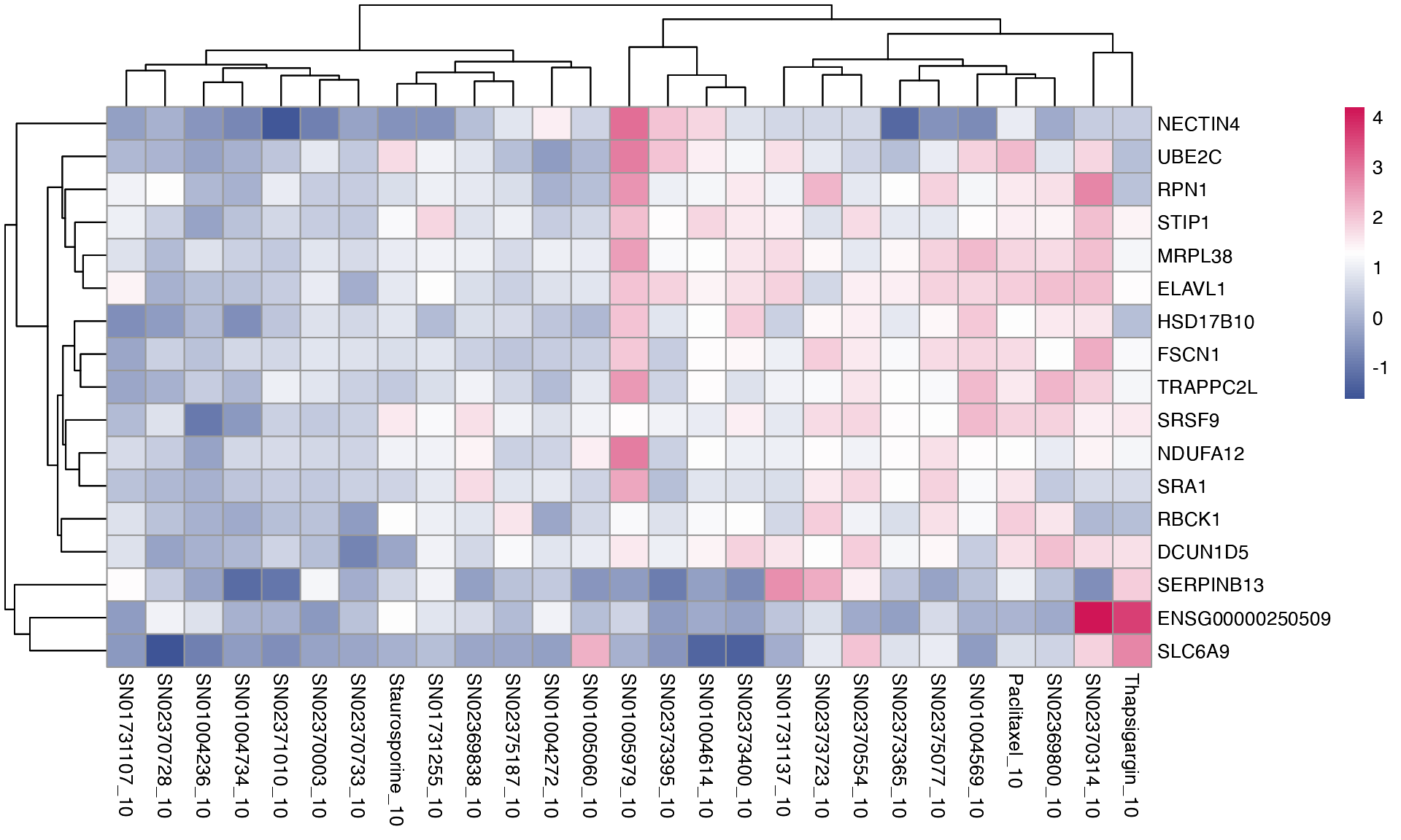
If you prefer to see the expression level on replicate level, you can specify logCPM = “lcpm”. Since we are observing log CPM of individual samples, and not the comparisons, we can also visualise the DMSO control.
plot_multi_de(mac, group_by = "combined_id", value = "lcpm", p_value_cutoff = 0.01, direction="up", n_genes = 5, control = "DMSO_0", by="fc")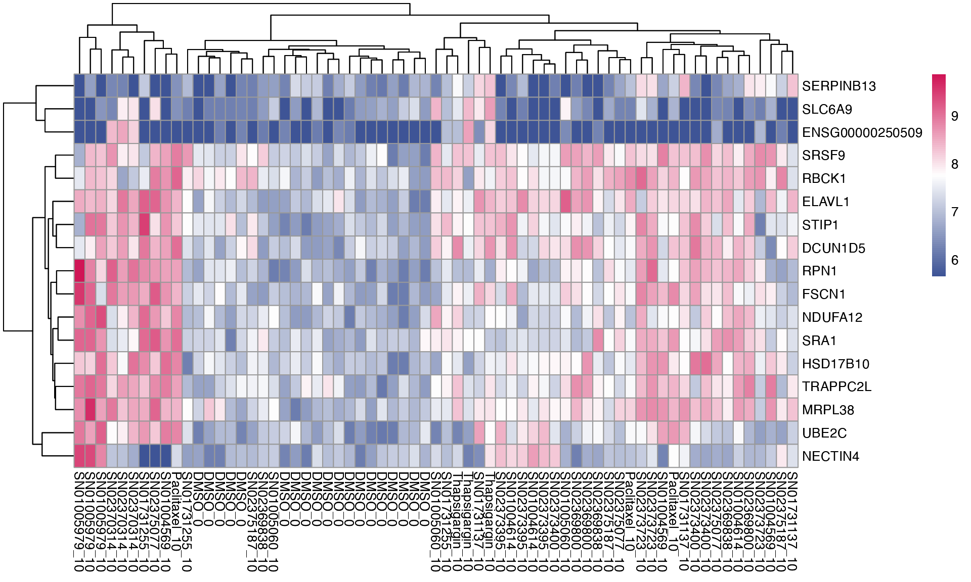
The outputs from the analyses above can be represented in table format.
summarise_de(mac, lfc_threshold = 1, padj_threshold = 0.01, multi=TRUE)
#> # A tibble: 27 × 7
#> combined_id Total_genes_tested Significantly_upregu…¹ Significantly_downre…²
#> <chr> <int> <int> <int>
#> 1 Paclitaxel_… 5660 629 91
#> 2 SN01004236_… 5660 0 0
#> 3 SN01004272_… 5660 1 0
#> 4 SN01004569_… 5660 257 49
#> 5 SN01004614_… 5660 220 36
#> 6 SN01004734_… 5660 0 0
#> 7 SN01005060_… 5660 13 4
#> 8 SN01005979_… 5660 936 853
#> 9 SN01731107_… 5660 4 3
#> 10 SN01731137_… 5660 148 69
#> # ℹ 17 more rows
#> # ℹ abbreviated names: ¹Significantly_upregulated, ²Significantly_downregulated
#> # ℹ 3 more variables: Total_significant <int>, padj_threshold <dbl>,
#> # Log2FC_threshold <dbl>3.4. Pathway analysis - multiple comparisons
Pathway enrichment analysis can then also be performed across all treatments, and summarised in a heatmap.
# Load genesets from enrichr for a specific species or define your own
enrichr_genesets <- download_geneset("human", "MSigDB_Hallmark_2020")
mac <- compute_multi_enrichr(mac, genesets = enrichr_genesets)

enriched_pathways_mat <- mac@tools$pathway_enrichment %>%
  bind_rows() %>%
  select(combined_id, Term, Combined.Score) %>%
  pivot_wider(names_from = combined_id, values_from = Combined.Score) %>%
  column_to_rownames(var = "Term") %>%
  mutate(across(everything(), ~ ifelse(is.na(.), 0, log1p(.)))) %>%  # Replace NA with 0 across all columns
  as.matrix()


pheatmap(enriched_pathways_mat, color = macpie_colours$continuous_rev)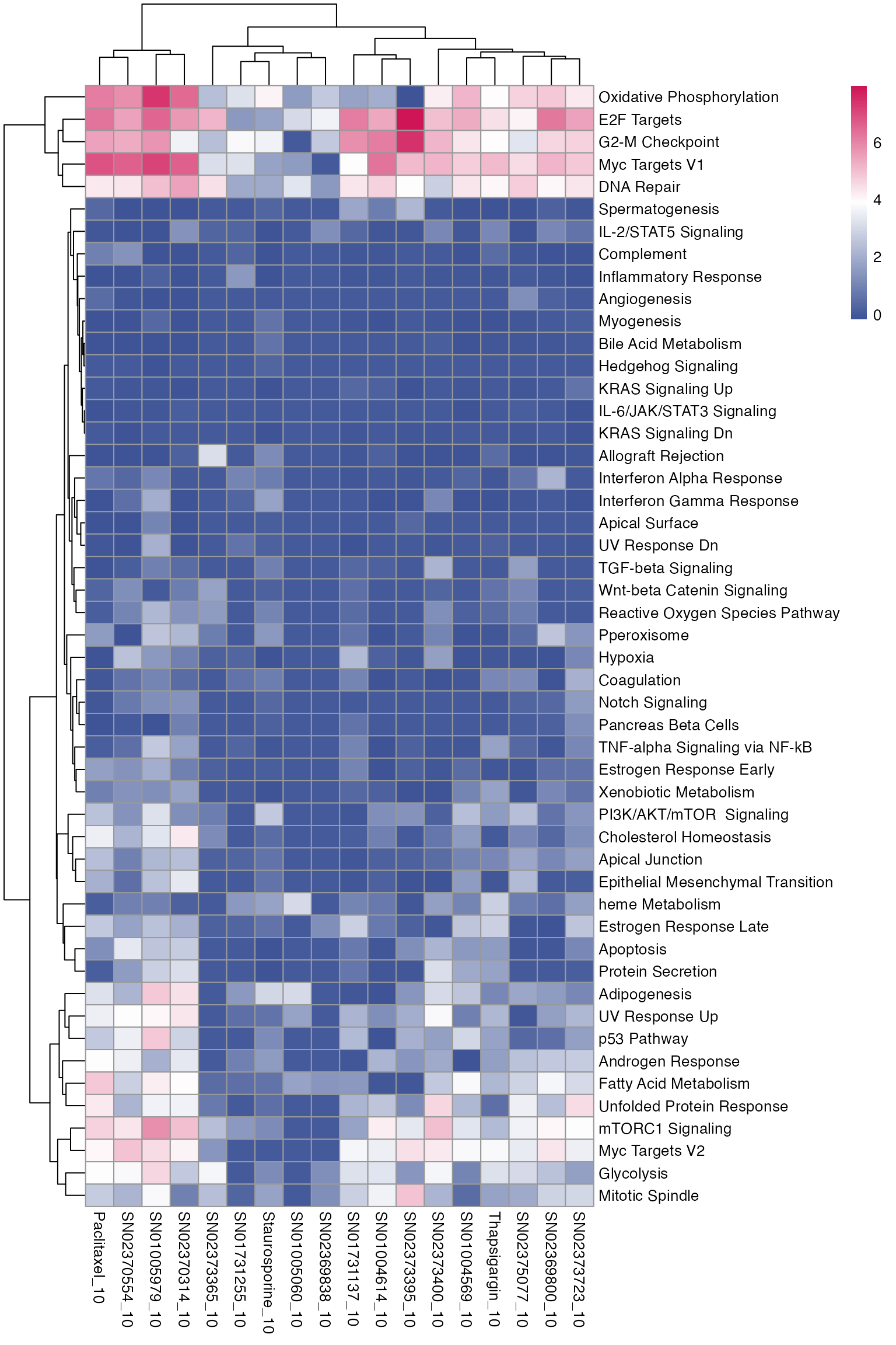
Quick check of some treatments:
Nutlin.3a is a MDM2-P53 inhibitor and stablises the p53 protein. It induces cell autophagy and apotopsis. Nutlin-activated p53 induces G1 and G2 arrest in cancer cell lines (see in the pathway enrichment heatmap).
Ref: Tovar C, et al. Proc Natl Acad Sci USA. 2006;103(6):1888–1893. Shows Nutlin-3’s effect on various p53 targets in cancer cell lines.