Cross platform compatibility

Introduction

This vignette is to demonstrate how to adapt macpie’s MACseq workflows to any high-throughput transcriptomic profiling (HTTr) data format such as DRUGseq. As the experimental design of DRUGseq plates is a bit different from MACseq. In MACseq experimental design, we prefer to have replicate wells in the same plate. While in DRUGseq, the replicates are in different plates.

Key points:

This vignette will cover the following two parts:

1. Converting a DRUGseq plate

Mapping DRUGseq plate layouts into macpie’s metadata format.
Validating the metadata format and content.
Some basic QC steps from QC vignette.

2. Converting multiple DRUGseq plates

Importing multiple plates into a single macpie object.
Detecting batch effects across plates in the QC section.
Performing differential expression and pathway enrichment tests on merged data with limma-voom correction.

3. Benchmark

Benchmarking the performance of macpie functions on DRUGseq data. It includes both filtering robust DMSO controls and DEG concordance.

The DRUGseq dataset is a large-scale drug screening dataset that includes a large set of small molecules (N = 4,343) tested on U2OS cells. This dataset was retrieved from Zenodo (Ozer et al., 2024).

suppressMessages(library(macpie))
suppressMessages(library(tibble))
suppressMessages(library(stringr))
suppressMessages(library(pheatmap))
suppressMessages(library(ggiraph))
suppressMessages(library(tidyseurat))
suppressMessages(library(purrr))
suppressMessages(library(ggrepel))

options(scipen=999, digits=3)

Converting a DRUGseq plate to a macpie object

1. Metadata import and validation

Experimental background and metadata files are in Novartis_drugseq_U2OS_MoABox/ on DRUGseq Github and data can be downloaded from this ZENODO link: Novartis/DRUG-seq U2OS MoABox Dataset Creators.

plate_well_metadata <- read.csv(paste0(dir,"DRUGseqData/DRUGseq_U2OS_MoABox_plate_wells_metadata_public.txt"), sep = "\t")

As the metadata contains plate and well-level information for the 59,904 samples, we only read in the metadata for plate VH02012944, which is the plate we use in this vignette.

metadata <- plate_well_metadata%>%filter(plate_barcode == "VH02012944")

1.1 Convert DRUGseq metadata to macpie metadata format

An example of a DRUGseq plate content format is also available on on DRUGseq Github.

First, we can have a look at the content and column names:

head(metadata)
#>   analysis_id investigation_id    investigation_name batch_id plate_replicate
#> 1          24             2384 DRUG-seq_CBT_U2OS_MoA       24               2
#> 2          24             2384 DRUG-seq_CBT_U2OS_MoA       24               2
#> 3          24             2384 DRUG-seq_CBT_U2OS_MoA       24               2
#> 4          24             2384 DRUG-seq_CBT_U2OS_MoA       24               2
#> 5          24             2384 DRUG-seq_CBT_U2OS_MoA       24               2
#> 6          24             2384 DRUG-seq_CBT_U2OS_MoA       24               2
#>   experiment_id              plate_name plate_barcode plate_index well_id
#> 1          6487 U-2_OS_MoA_batch24_rep2    VH02012944    TTACAGGA     A01
#> 2          6487 U-2_OS_MoA_batch24_rep2    VH02012944    TTACAGGA     J01
#> 3          6487 U-2_OS_MoA_batch24_rep2    VH02012944    TTACAGGA     K01
#> 4          6487 U-2_OS_MoA_batch24_rep2    VH02012944    TTACAGGA     L01
#> 5          6487 U-2_OS_MoA_batch24_rep2    VH02012944    TTACAGGA     M01
#> 6          6487 U-2_OS_MoA_batch24_rep2    VH02012944    TTACAGGA     N01
#>   well_index col row well_type cell_line_name cell_line_ncn concentration unit
#> 1 AACAAGGTAC   1   1        SA         U-2 OS     FH55-48QE            10   uM
#> 2 AAGATCGGCG   1  10        SA         U-2 OS     FH55-48QE            10   uM
#> 3 AAGCGATGTT   1  11        SA         U-2 OS     FH55-48QE            10   uM
#> 4 AAGCGTTCAG   1  12        SA         U-2 OS     FH55-48QE            10   uM
#> 5 AAGGTCTGGA   1  13        SA         U-2 OS     FH55-48QE            10   uM
#> 6 AAGTTAGCGC   1  14        SA         U-2 OS     FH55-48QE            10   uM
#>   hours_post_treatment biosample_id external_biosample_id cmpd_sample_id
#> 1                   24      2018772            KA-74-VF86     BA-86-AL61
#> 2                   24      2018988            AB-94-KK84     BB-79-AG41
#> 3                   24      2019012            OD-91-CJ88     BB-41-XE67
#> 4                   24      2019036            AE-90-GO84     ED-91-LA02
#> 5                   24      2019060            MF-99-JS89     DF-11-IL69
#> 6                   24      2019084            UB-01-LS89     LE-80-BM08
#>              plate_well
#> 1 VH02012944_AACAAGGTAC
#> 2 VH02012944_AAGATCGGCG
#> 3 VH02012944_AAGCGATGTT
#> 4 VH02012944_AAGCGTTCAG
#> 5 VH02012944_AAGGTCTGGA
#> 6 VH02012944_AAGTTAGCGC

Next, we convert relevant columns in DRUGseq metadata to macpie metadata format.

#extract relevant columns from DRUGseq plate 
macpie_metadata <- metadata %>%
  select(plate_barcode, well_id, well_index, row, col, well_type, cell_line_name, concentration, unit, hours_post_treatment, cmpd_sample_id) %>%
  mutate(
    Plate_ID = plate_barcode,
    Well_ID = well_id,
    Barcode = well_index,
    Cell_type = "U2OS",
    Unit_1 = unit, 
    Treatment_1 = cmpd_sample_id,
    Sample_type = well_type,
    Concentration_1 = as.numeric(concentration),
    Row = LETTERS[row],
    Column = as.integer(col),
    Time = as.factor(hours_post_treatment),
    Unit = "h",
    Species = "human",
    Model_type = "2D_adherent",
    Sample_type = if_else(well_type == "SA" & col == 24,
                                  "Positive Control",
                                  well_type)

)

#Column names for macpie
col_names <- c("Plate_ID", "Well_ID", "Row", "Column", "Species",
               "Cell_type",  "Model_type", "Time", "Unit", "Treatment_1", 
               "Concentration_1", "Unit_1",  "Sample_type", "Barcode")
macpie_metadata <- macpie_metadata[, col_names]

head(macpie_metadata)
#>     Plate_ID Well_ID Row Column Species Cell_type  Model_type Time Unit
#> 1 VH02012944     A01   A      1   human      U2OS 2D_adherent   24    h
#> 2 VH02012944     J01   J      1   human      U2OS 2D_adherent   24    h
#> 3 VH02012944     K01   K      1   human      U2OS 2D_adherent   24    h
#> 4 VH02012944     L01   L      1   human      U2OS 2D_adherent   24    h
#> 5 VH02012944     M01   M      1   human      U2OS 2D_adherent   24    h
#> 6 VH02012944     N01   N      1   human      U2OS 2D_adherent   24    h
#>   Treatment_1 Concentration_1 Unit_1 Sample_type    Barcode
#> 1  BA-86-AL61              10     uM          SA AACAAGGTAC
#> 2  BB-79-AG41              10     uM          SA AAGATCGGCG
#> 3  BB-41-XE67              10     uM          SA AAGCGATGTT
#> 4  ED-91-LA02              10     uM          SA AAGCGTTCAG
#> 5  DF-11-IL69              10     uM          SA AAGGTCTGGA
#> 6  LE-80-BM08              10     uM          SA AAGTTAGCGC

1.2 Validate DRUGseq metadata

Now, we can test the metadata validation function to ensure that the metadata is in the correct format and contains all the required columns.

validate_metadata(macpie_metadata)
#> 
#> No validation issues found. Metadata is clean.
#> 
#> Generating summary table grouped by Plate_ID...
#>     Plate_ID count_Species count_Cell_type count_Model_type count_Time
#> 1 VH02012944             1               1                1          1
#>   count_Unit count_Treatment_1 count_Concentration_1 count_Unit_1
#> 1          1               341                     2            1
#>   count_Sample_type
#> 1                 4

Visualizing and inspecting the metadata layout

plot_metadata_heatmap(macpie_metadata)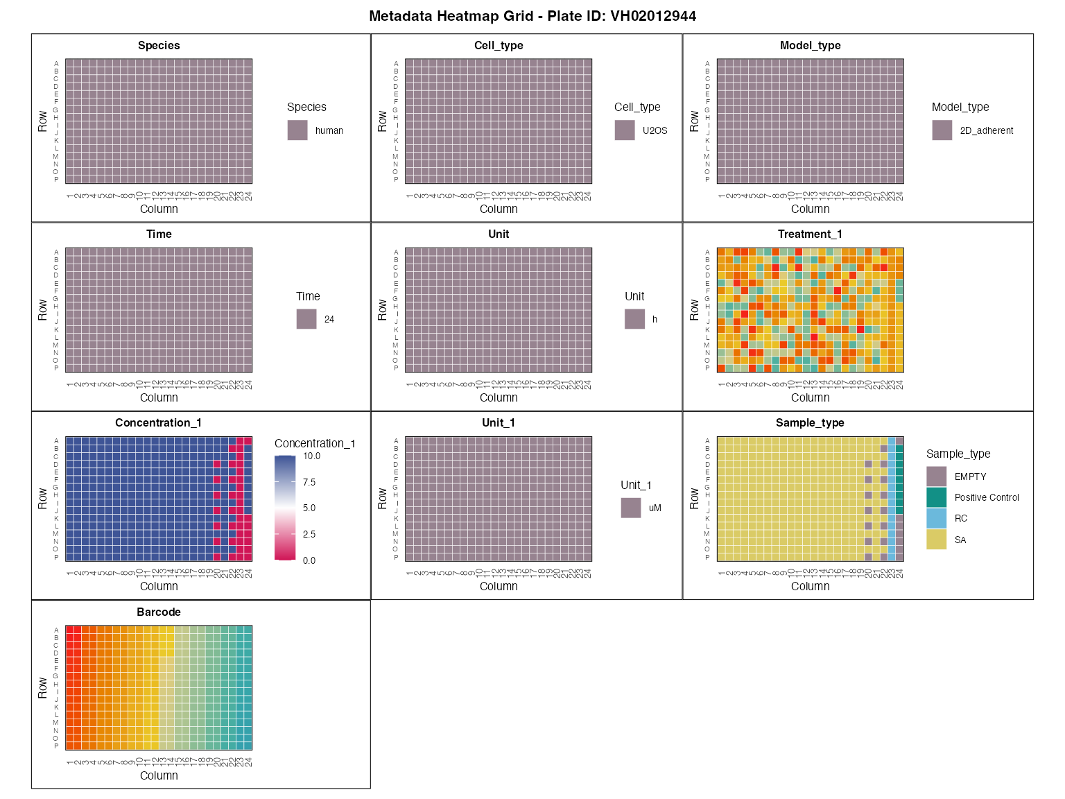

2. Quality control

2.1 Import data

Let’s import one of the replicate plates VH02012944 from batch 24.

DRUGseq data was downloaded from ./Exp_gzip.RData from the above Zenodo link and saved as Exp_batch24.Rds locally for faster loading.

Each batch is a list of plates, and each plate contains the UMI counts matrix and the corresponding metadata.

# load("DRUGseqData/Exp_gzip.RData")
# batch24 <- Exp$`24`
# saveRDS(batch24, file = "DRUGseqData/Exp_batch24.Rds")
batch24 <- readRDS(paste0(dir,"DRUGseqData/Exp_batch24.Rds"))

data <- batch24$VH02012944
counts <- data$UMI.counts
colnames(counts) <- str_remove_all(colnames(counts), "VH02012944_")

Quick check of the UMI counts matrix dimensions and the first few row names:

dim(data$UMI.counts)
#> [1] 59594   384
rownames(data$UMI.counts)[1:10]
#>  [1] "DUX4L9,grch38_4"      "AC010378.2,grch38_5"  "AL136295.5,grch38_14"
#>  [4] "AC106786.1,grch38_5"  "AC138956.2,grch38_5"  "MTND2P40,grch38_19"  
#>  [7] "AC104109.2,grch38_5"  "RNU6-1263P,grch38_3"  "AC243972.3,grch38_14"
#> [10] "COX6B1P5,grch38_4"

Row names of DRUGseq data are in the format of “gene_chromosome”. But we only keep gene names for macpie data.

counts <- rownames_to_column(as.data.frame(counts), var= "gene_id") %>%
  separate(gene_id, into = c("gene_name", "chrom"), sep = ",") 
counts[1:10,1:5]
#>     gene_name     chrom CGGAGATTGG ACACCGAATT AGCCACTAGC
#> 1      DUX4L9  grch38_4          0          0          0
#> 2  AC010378.2  grch38_5          0          0          0
#> 3  AL136295.5 grch38_14          4          2          9
#> 4  AC106786.1  grch38_5          0          0          0
#> 5  AC138956.2  grch38_5          0          0          0
#> 6    MTND2P40 grch38_19          0          0          0
#> 7  AC104109.2  grch38_5          0          0          0
#> 8  RNU6-1263P  grch38_3          0          0          0
#> 9  AC243972.3 grch38_14          0          0          0
#> 10   COX6B1P5  grch38_4          0          0          0

counts$gene_name <- make.unique(counts$gene_name)
counts <- counts %>%
  select(-chrom) %>%
  tibble::column_to_rownames(var = "gene_name")  %>%
  as.matrix()

The UMI counts matrix and metadata are now ready to be used with macpie functions. We can create a tidySeurat object and join it with the metadata.

as_mac<- CreateSeuratObject(counts = counts, 
                                     assay = "RNA", 
                                     project = "VH02012944")
#> Warning: Feature names cannot have underscores ('_'), replacing with dashes
#> ('-')
#> Warning: Data is of class matrix. Coercing to dgCMatrix.
as_mac<- as_mac%>% inner_join(macpie_metadata, by = c(".cell"="Barcode"))

Filtering:

We previously saved a filtered data set, which filtered out genes with < 5 reads in at least 1 replicate well for each treatment.

# as_mac <- filter_genes_by_expression(as_mac, 
#                                      group_by = "Treatment_1",
#                                      min_counts = 5,
#                                      min_samples = 1)
as_mac <- readRDS(paste0(dir, "/DRUGseqData/macpie_filtered_VH02012944.rds"))

2.2 Visualize plate layout

Now, we can check UMI counts and sample types in the wells.

p <- plot_plate_layout(as_mac, "nCount_RNA", "Sample_type")
girafe(ggobj = p, 
  fonts = list(sans = "sans"),
  options = list(
    opts_hover(css = "stroke:black; stroke-width:0.8px;")  # <- slight darkening
  ))

We can check common QC plots from the Seurat package to visualise the number of genes, reads, and percentage of mitochondrial and ribosomal genes per sample.

# Calculate percent of mitochondrial and ribosomal genes
as_mac[["percent.mt"]] <- PercentageFeatureSet(as_mac, pattern = "^mt-|^MT-")
as_mac[["percent.ribo"]] <- PercentageFeatureSet(as_mac, pattern = "^Rp[slp][[:digit:]]|^Rpsa|^RP[SLP][[:digit:]]|^RPSA")

# Example of a function from Seurat QC 
VlnPlot(as_mac, features = c("nFeature_RNA", "nCount_RNA", "percent.mt", "percent.ribo"), 
        ncol = 4, group.by = "Sample_type") & 
  scale_fill_manual(values = macpie_colours$discrete) 
#> Warning: Default search for "data" layer in "RNA" assay yielded no results;
#> utilizing "counts" layer instead.
#> Warning: The `slot` argument of `FetchData()` is deprecated as of SeuratObject 5.0.0.
#> ℹ Please use the `layer` argument instead.
#> ℹ The deprecated feature was likely used in the Seurat package.
#>   Please report the issue at <https://github.com/satijalab/seurat/issues>.
#> This warning is displayed once every 8 hours.
#> Call `lifecycle::last_lifecycle_warnings()` to see where this warning was
#> generated.
#> Warning: `PackageCheck()` was deprecated in SeuratObject 5.0.0.
#> ℹ Please use `rlang::check_installed()` instead.
#> ℹ The deprecated feature was likely used in the Seurat package.
#>   Please report the issue at <https://github.com/satijalab/seurat/issues>.
#> This warning is displayed once every 8 hours.
#> Call `lifecycle::last_lifecycle_warnings()` to see where this warning was
#> generated.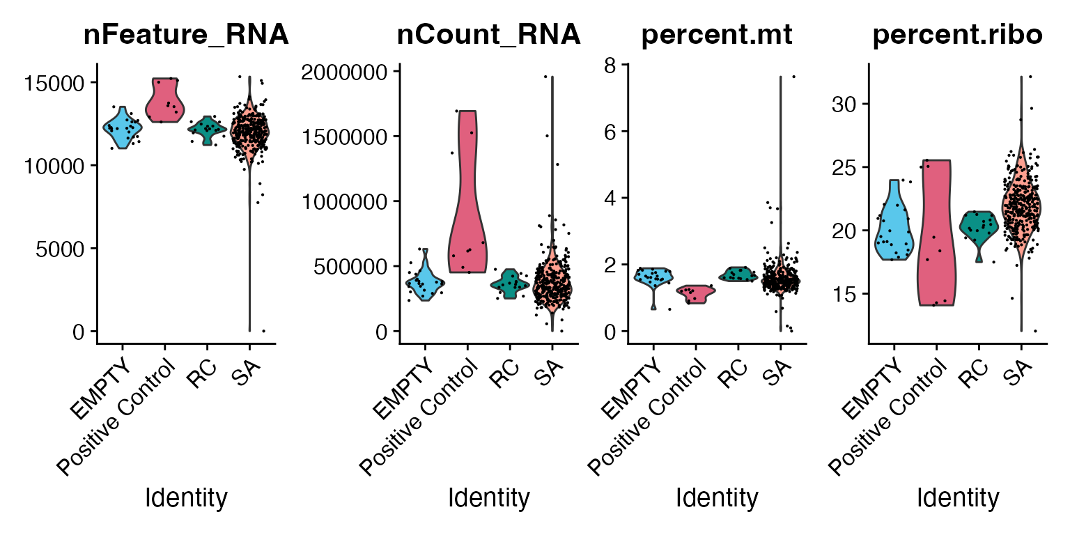

2.2 Basic QC metrics

2.2.1 Sample grouping

Same as the Quality control vignette, we first visualise grouping of the samples based on top 500 expressed genes and limma’s MDS function. Hovering over the individual dots reveals sample identity and grouping.

p <- plot_mds(as_mac, group_by = "Sample_type", label = "Sample_type", n_labels = 30)
#> tidyseurat says: Key columns are missing. A data frame is returned for independent data analysis.
#> tidyseurat says: Key columns are missing. A data frame is returned for independent data analysis.
girafe(ggobj = p, fonts = list(sans = "sans"))
#> Warning: ggrepel: 7 unlabeled data points (too many overlaps). Consider
#> increasing max.overlaps

2.2.2 Correction of the batch effect

For simplicity, we only plot the RLE (Relative Log Expression) plot for different types of controls.

plot_rle(as_mac %>% filter(Sample_type !="SA"), label_column = "Sample_type", normalisation = "raw")
#> tidyseurat says: Key columns are missing. A data frame is returned for independent data analysis.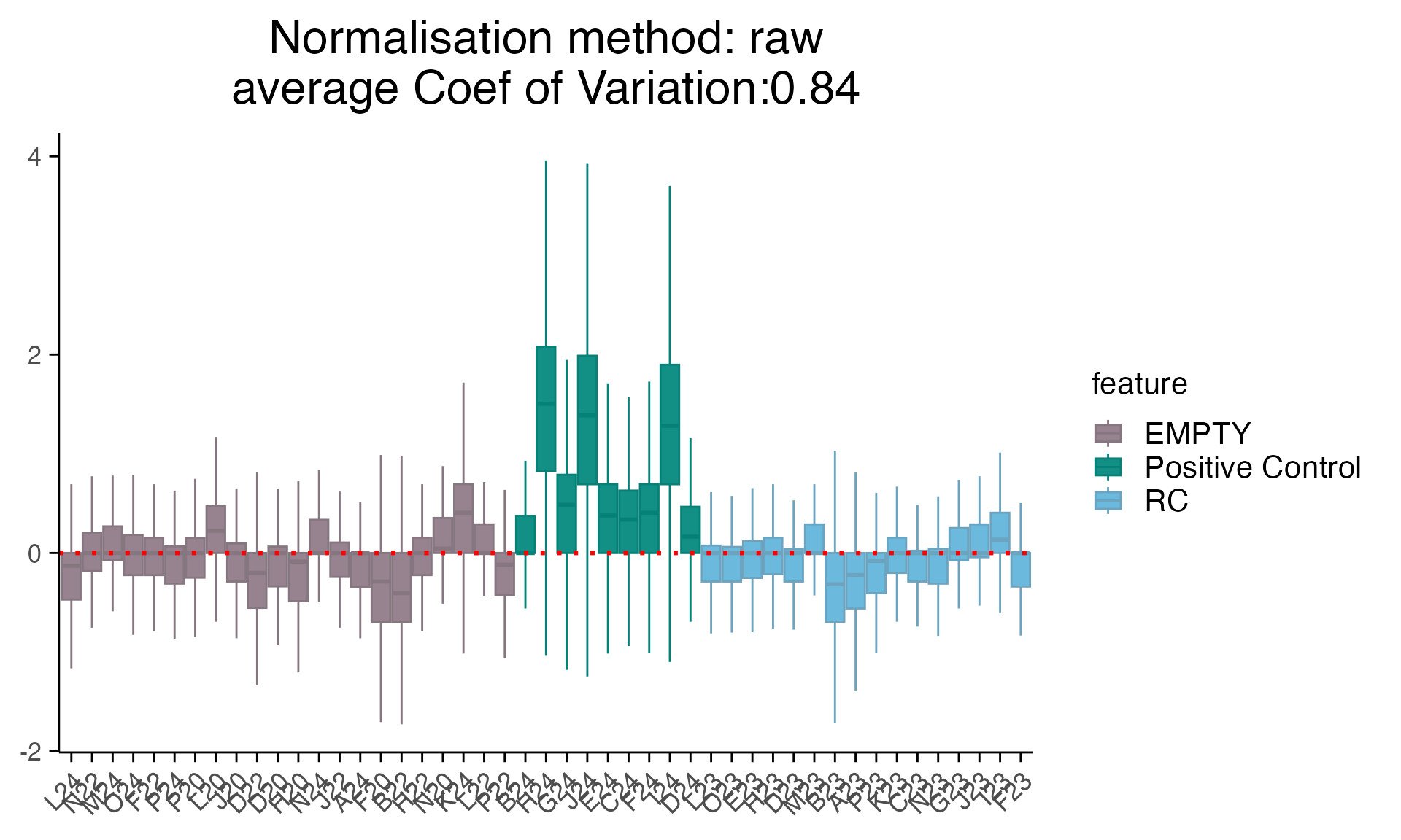

plot_rle(as_mac %>% filter(Sample_type !="SA"), label_column = "Sample_type", normalisation = "limma_voom")
#> tidyseurat says: Key columns are missing. A data frame is returned for independent data analysis.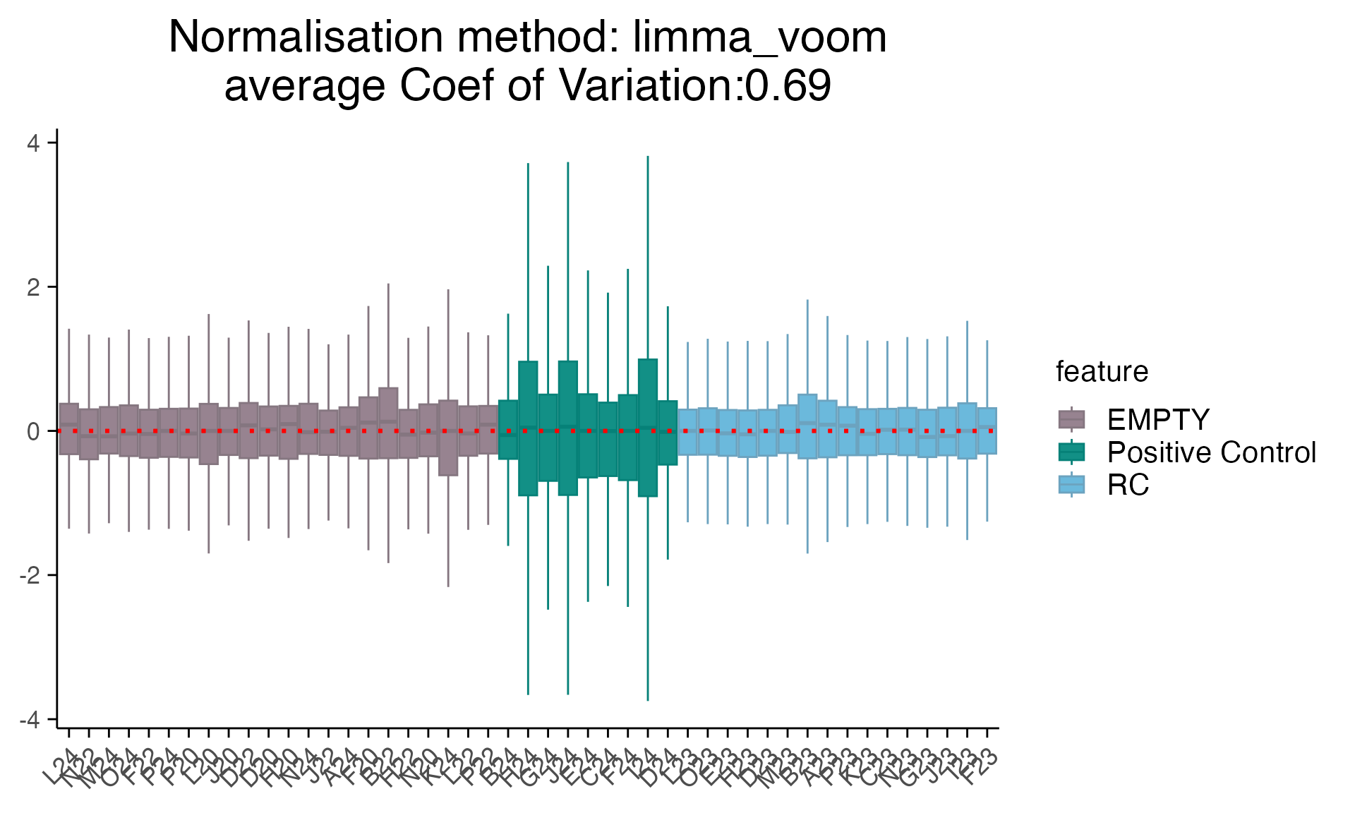

Coverting multiple DRUGseq plates to a macpie object

1. Metadata import and validation

In this part of the vignette, we need three replicate plates from batch 24.

DRUGseq data was downloaded from ./Exp_gzip.RData from the above Zenodo link and saved as Exp_batch24.Rds locally for faster loading.

Each batch is a list of plates, and each plate contains the UMI counts matrix and the corresponding metadata.

names(batch24)
#> [1] "VH02012956" "VH02012942" "VH02012944"

This batch contains 3 replicate plates, each has the UMI counts matrix and the metadata.

Now, we convert the metadata format to macpie metadata format.

The idea is to make a combined metadata and a combined count matrix for three plates with the plate_ID labelled.

#make a combined metadata for three plates
batch24_metadata <- batch24 %>% 
  map_dfr(~ {
    .x$Annotation %>%
      mutate(
        Plate_ID        = plate_barcode,
        Well_ID         = well_id,
        Barcode         = paste0(plate_barcode, "_", well_index),
        Row             = LETTERS[row],
        Column          = as.integer(col),
        Species         = "human",
        Cell_type       = "U2OS",
        Model_type      = "2D_adherent",
        Time            = as.factor(hours_post_treatment),
        Unit            = "h",
        Treatment_1     = cmpd_sample_id,
        Concentration_1 = as.numeric(concentration),
        Unit_1          = unit,
        Sample_type     = if_else(well_type == "SA" & col == 24,
                                  "Positive Control",
                                  well_type)
      )
  })


batch24_metadata <- batch24_metadata%>%select(-c(batch_id, plate_barcode,plate_index, well_id,
                                                 well_index, col, row, biosample_id, external_biosample_id,
                                                 cmpd_sample_id, well_type, cell_line_name, cell_line_ncn, concentration, unit, hours_post_treatment, Sample))

# create a combined UMI matrix for 3 plates
batch24_counts <- batch24 %>%
  map(~ {
    .x$UMI.counts %>%
      as.data.frame() %>% 
      rownames_to_column("gene_id") %>%
      separate(col = gene_id, into = c("gene_name", "chrom"), sep = ",") %>%
      mutate(gene_name = make.unique(gene_name)) %>%
      select(-chrom) %>%
      tibble::column_to_rownames(var = "gene_name") %>%
      as.matrix()
  })

binded_counts <- do.call(cbind, batch24_counts)

2. Quality control

2.1 Import data

Then, we can read in the combined count matrix and metadata.

as_mac <- CreateSeuratObject(counts = binded_counts, 
  min.cells = 1, 
  min.features = 1)
#> Warning: Feature names cannot have underscores ('_'), replacing with dashes
#> ('-')
#> Warning: Data is of class matrix. Coercing to dgCMatrix.

as_mac<- as_mac%>% inner_join(batch24_metadata, by = c(".cell"="Barcode"))

Filtering

As filtering genes in three 384-well plates could take a while. We suggest to save a previously filtered object to work with.

as_mac$combined_id <- paste0(as_mac$Treatment_1,"_", as_mac$Concentration_1)

min_sample_num <- min(table(as_mac$combined_id))

# mac_filtered <- filter_genes_by_expression(as_mac, 
#                                            group_by = "combined_id", min_counts = 10,
#                                            min_samples = min_sample_num)
# 
# saveRDS(mac_filtered, 
#   file = paste0(dir, "DRUGseqData/macpie_filtered_batch24.Rds"))


mac_filtered <- readRDS(paste0(dir, "/DRUGseqData/macpie_filtered_batch24.Rds"))

Here, we focus on check the data quality across three replicate plates, especially any batch effects from this batch 24.

mac_filtered[["percent.mt"]] <- PercentageFeatureSet(mac_filtered, pattern = "^mt-|^MT-")
mac_filtered[["percent.ribo"]] <- PercentageFeatureSet(mac_filtered, pattern = "^Rp[slp][[:digit:]]|^Rpsa|^RP[SLP][[:digit:]]|^RPSA")
# Example of a function from Seurat QC 
VlnPlot(mac_filtered, features = c("nFeature_RNA", "nCount_RNA", "percent.mt", "percent.ribo"), 
        ncol = 4, group.by = "Sample_type", split.by = "orig.ident") + theme(legend.position = 'right') +
  scale_fill_manual(values = macpie_colours$discrete) 
#> Warning: Default search for "data" layer in "RNA" assay yielded no results;
#> utilizing "counts" layer instead.
#> The default behaviour of split.by has changed.
#> Separate violin plots are now plotted side-by-side.
#> To restore the old behaviour of a single split violin,
#> set split.plot = TRUE.
#>       
#> This message will be shown once per session.
#> Scale for fill is already present.
#> Adding another scale for fill, which will replace the existing scale.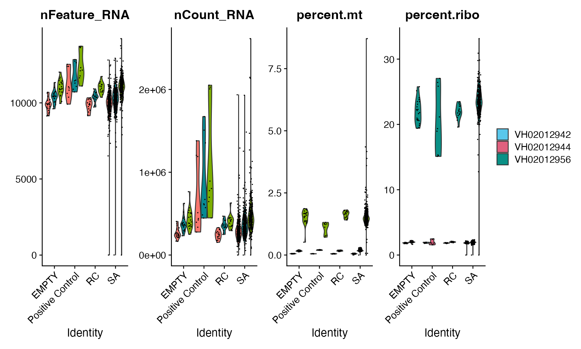

p <- plot_plate_layout(mac_filtered, "nCount_RNA", "combined_id") + facet_wrap(~orig.ident, ncol = 1) + 
  theme(strip.text = element_text(size=10),
        axis.text.x = element_text(size=10), 
        axis.text.y = element_text(size=8),
        legend.title = element_text(size=10),
        legend.text = element_text(size=8),
        trip.background = element_blank())
girafe(ggobj = p, 
  fonts = list(sans = "sans"),
  options = list(
    opts_hover(css = "stroke:black; stroke-width:1px;")
  ))
#> Warning in plot_theme(plot): The `trip.background` theme element is not
#> defined in the element hierarchy.

2.2 Basic QC metrics

2.2.1 Sample grouping with MDS plot

Same as above, we first visualise grouping of the samples in MDS plot.

p <- plot_mds(mac_filtered, group_by = "Sample_type", label = "combined_id", n_labels = 30)
#> tidyseurat says: Key columns are missing. A data frame is returned for independent data analysis.
#> tidyseurat says: Key columns are missing. A data frame is returned for independent data analysis.

p1 <- plot_mds(mac_filtered, group_by = "orig.ident", label = "combined_id", n_labels = 30)
#> tidyseurat says: Key columns are missing. A data frame is returned for independent data analysis.
#> tidyseurat says: Key columns are missing. A data frame is returned for independent data analysis.


g <- patchwork::wrap_plots(list(p, p1), ncol = 1, nrow = 2, rel_widths = c(7, 7), rel_heights = c(10, 10))
girafe(
  ggobj      = g, 
  width_svg  = 10,    # 10 inches wide
  height_svg = 10,     #  10 inches tall
  fonts      = list(sans = "sans"),
  options    = list(opts_hover(css = "stroke:black; stroke-width:0.8px;"))
)
#> Warning: ggrepel: 30 unlabeled data points (too many overlaps). Consider increasing max.overlaps
#> ggrepel: 30 unlabeled data points (too many overlaps). Consider increasing max.overlaps

2.2.2 Sample grouping with UMAP

Apart from MDS plot, we show that this data can also be applied to Seurat’s SCTransform to visualise in UMAP.

mac_sct <- SCTransform(mac_filtered, verbose = FALSE) %>%
    RunPCA(verbose = FALSE) %>%
    RunUMAP(verbose = FALSE,dims = 1:30)

DimPlot(mac_sct, reduction = "umap", group.by = "orig.ident", cols = macpie_colours$discrete)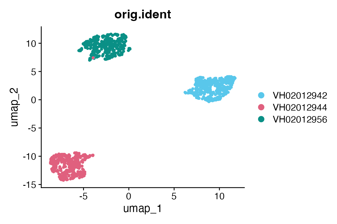

From MDS and UMAP, there are batch effects among three replicate plates. Only one compound: three wells of BA-51-N076_10 formed a distinct cluster. All wells were separated by plates.

2.2.3 Distribution of UMI counts

We also want to expect what is the distribution of UMIs across the experiment. To that end we use box plot to show distribution of UMI counts grouped across treatments.

length(unique(mac_filtered$combined_id))
#> [1] 341

As there are 341 unique combinations of compound_concentration, it’s too messy to show in the vignette. In here, we only show 200 of them.

compounds_subset <- unique(mac_filtered$combined_id)
qc_stats <- compute_qc_metrics(mac_filtered %>% filter(combined_id %in% compounds_subset[1:200]), group_by = "combined_id", order_by = "median")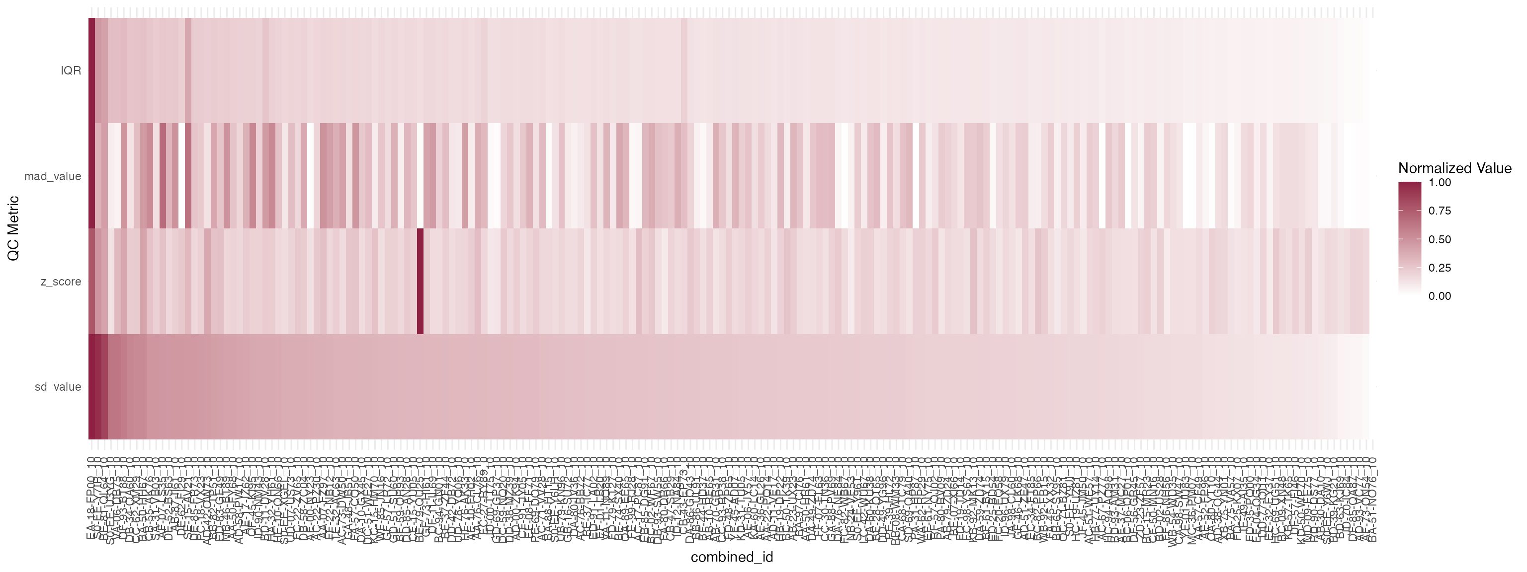

2.2.4 Variability among all replicates

plot_qc_metrics_heatmap(qc_stats$stats_summary)

2.2.5 Correction of batch effect

According to DRUGseq metadata:

Wells with water are labelled as EC-27-RY89
Wells with DMSO are labelled as CB-43-EP73

mac_filtered_dmso <- mac_filtered %>% filter(Treatment_1 == "CB-43-EP73")
plot_rle(mac_filtered_dmso, label_column = "orig.ident", normalisation = "raw")+ scale_x_discrete(drop = FALSE) + 
  theme(axis.text.x = element_text(angle = 45, hjust = 1))
#> tidyseurat says: Key columns are missing. A data frame is returned for independent data analysis.
#> Scale for x is already present.
#> Adding another scale for x, which will replace the existing scale.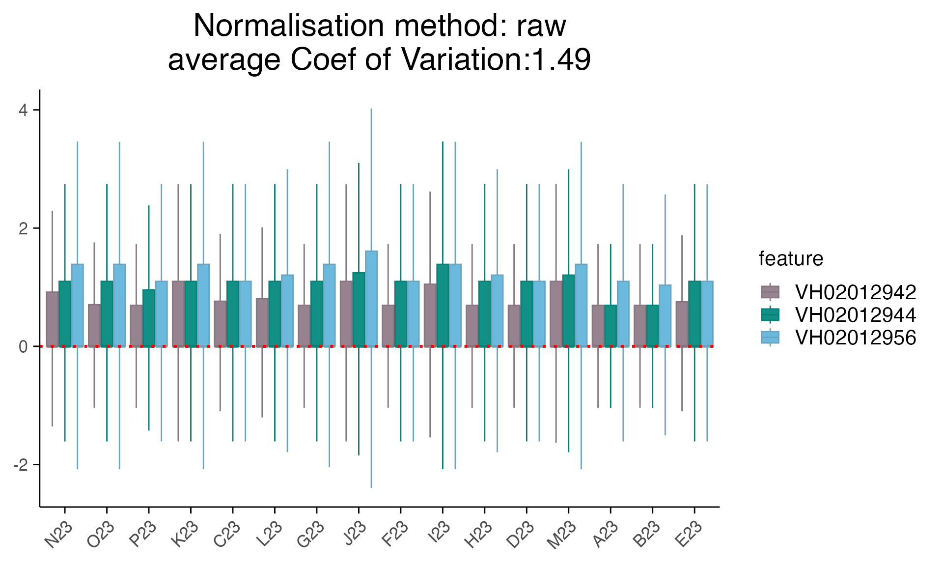

plot_rle(mac_filtered_dmso, label_column = "orig.ident", normalisation = "limma_voom")+ scale_x_discrete(drop = FALSE) + 
  theme(axis.text.x = element_text(angle = 45, hjust = 1))
#> tidyseurat says: Key columns are missing. A data frame is returned for independent data analysis.
#> Scale for x is already present.
#> Adding another scale for x, which will replace the existing scale.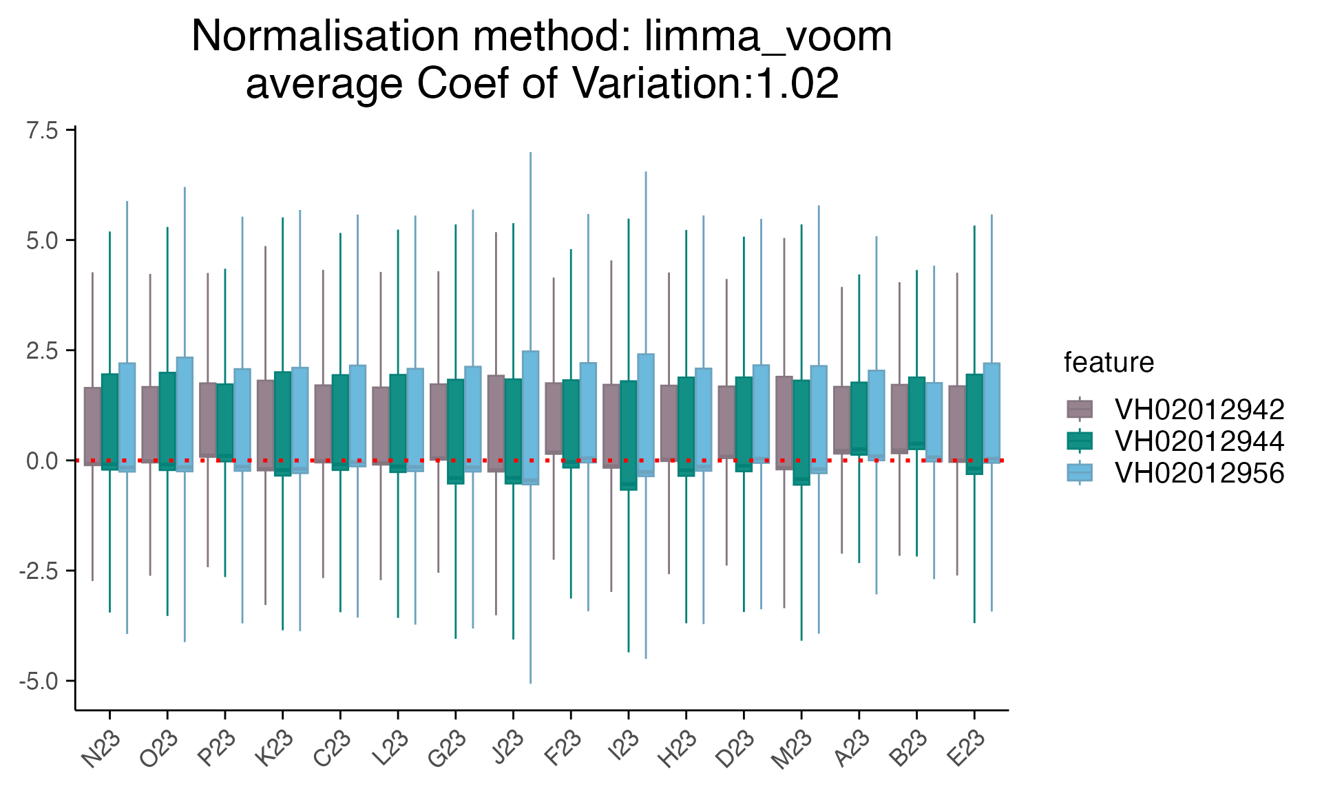

Note: instead of discussing which correction methods we should use for this data, we only show the ways we detected and corrected batch effect here. As batch effect adjustment for sequencing data has been implemented in different methods, such as DESeq2, RUVSeq, edgeR. We highly recommend users thoroughly checking any batch effects and exploring different methods.

In the next part of the vignette, we demonstrate a batch parameter has implemented in the differential expression test for batch correction.

3. Differential gene expression

3.1 Single comparison

In here, you can specify a single condition in the combined_id column and compare with DMSO (i.e.CB_43_EP73_0). By using the plate IDs in the column of orig.ident as the input for batch parameter, compute_singe_de function can perform differential expression analysis using the preferred method (limma voom in this example) with batch information.

mac_filtered$combined_id <- str_replace_all(mac_filtered$combined_id, "-","_")
treatment_samples <- "FF_86_NH56_10"
control_samples <- "CB_43_EP73_0"
subset <- mac_filtered%>%filter(combined_id%in%c(treatment_samples,control_samples))
batch <- subset$orig.ident
top_table <- compute_single_de(mac_filtered, treatment_samples, control_samples, method =  "limma_voom", batch = batch)
plot_volcano(top_table, max.overlaps = 6)
#> Warning: ggrepel: 5718 unlabeled data points (too many overlaps). Consider
#> increasing max.overlaps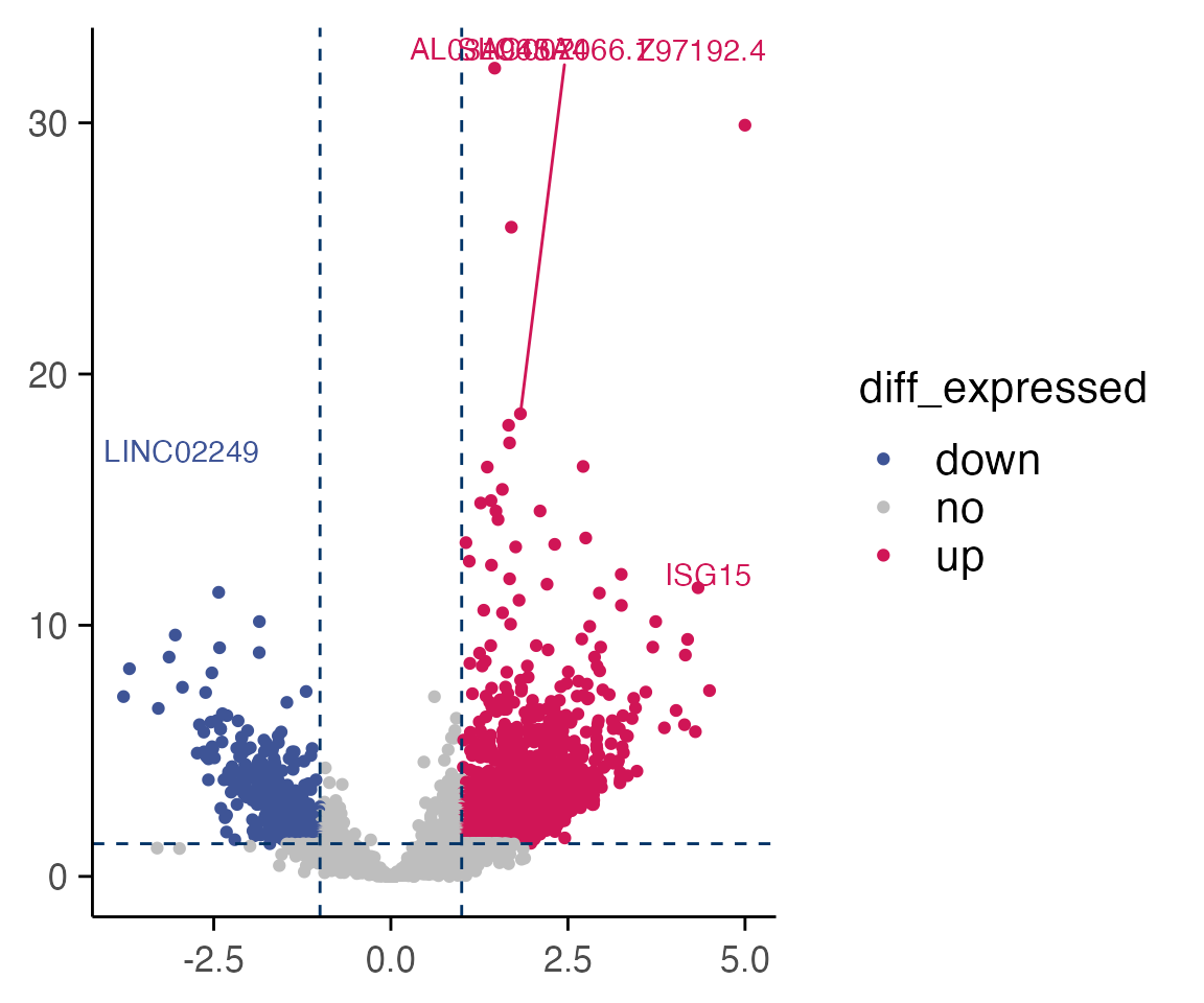

Now we can visualise gene expression (in CPM) for the top 6 genes from the differential expression analysis.

genes <- top_table$gene[1:6]
group_by <- "combined_id"
plot_counts(mac_filtered,genes, group_by, treatment_samples, control_samples, normalisation = "cpm")
#> Normalizing layer: counts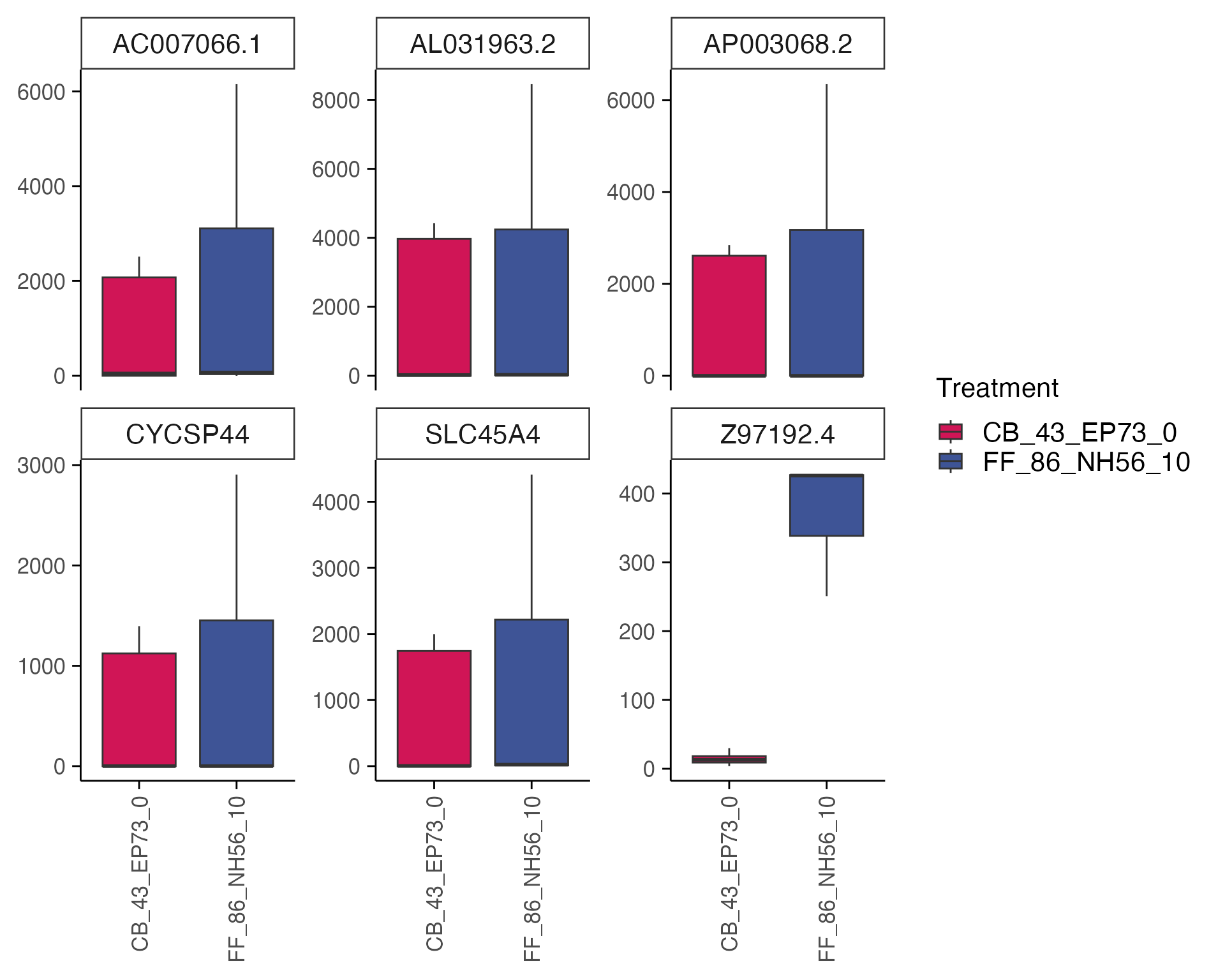

Pathway enrichment analysis can be performed on the top differentially expressed genes using function enrichr.

3.2 Multiple comparisons

As there are 339 compounds with 10uM in the data, which could take quite a while (around 24 mins for a M3 Pro 18GB memory on parallelisation speedup num_cores = 4) to run. For the purpose of this vignette, we only include 100 compounds with 10uM in the data.

treatments <- mac_filtered %>%
  filter(Concentration_1 == 10) %>%
  select(combined_id) %>%
  pull() %>%
  unique()
#> tidyseurat says: Key columns are missing. A data frame is returned for independent data analysis.

treatments_subset <- treatments[1:100] # only use 100 compounds for the vignette
  
mac_filtered <- compute_multi_de(mac_filtered, treatments_subset, control_samples = "CB_43_EP73_0", method = "limma_voom", num_cores = 4)

We often want to ask which genes are differentially expressed in more than one treatment group.

Here, we can visualise treatment groups with shared differentially expressed genes, defined as the top 20 up-regulated genes from each single drug comparison (treatment vs control) that are found in at least 2 different treatment groups.

The heatmap below shows shared differentially expressed genes with corresponding log2FC values.

plot_multi_de(mac_filtered, group_by = "combined_id", value = "log2FC", p_value_cutoff = 0.01, direction="up", n_genes = 20, control = "CB_43_EP73_0", by="fc")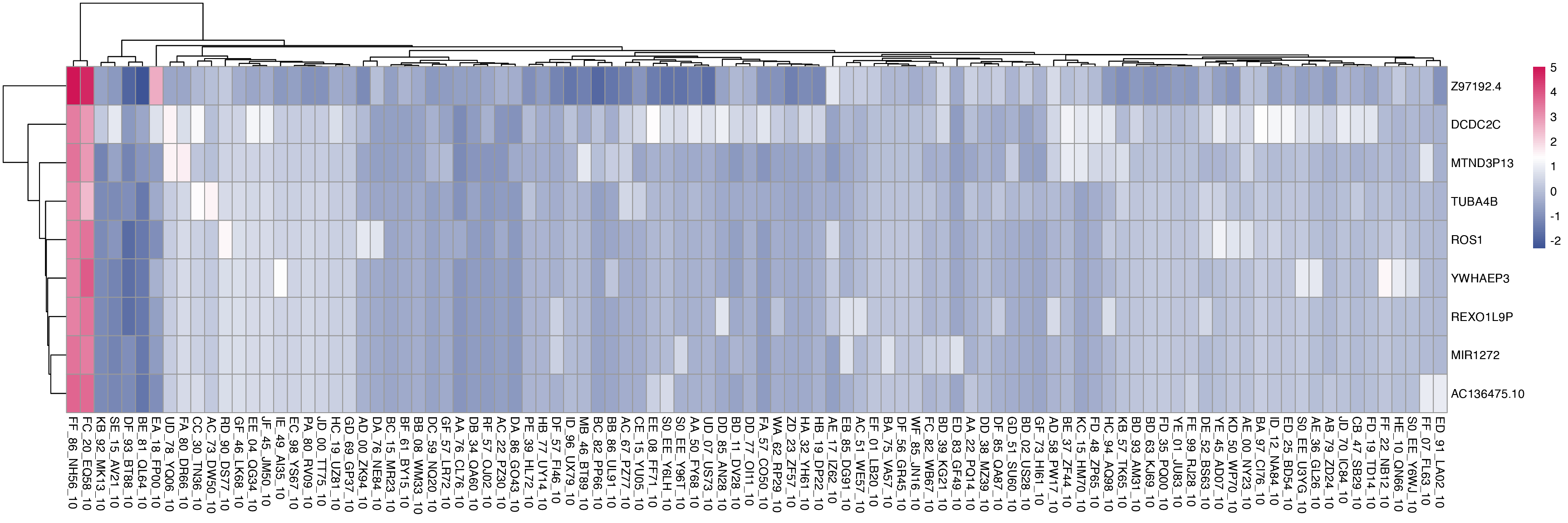

4. Pathway enrichment analysis

4.1 Multiple comparisons

The pathway enrichment analysis is done by using enrichR. Results from differential gene expression - multiple comparisons are used to pass on to the pathway enrichment analysis.

You can visualise the pathway enrichment results for multiple comparisons in a heatmap.

# Load genesets from enrichr for a specific species or define your own
enrichr_genesets <- download_geneset("human", "MSigDB_Hallmark_2020")
mac_filtered<- compute_multi_enrichr(mac_filtered, genesets = enrichr_genesets)

enriched_pathways_mat <- mac_filtered@tools$pathway_enrichment %>%
  bind_rows() %>%
  select(combined_id, Term, Combined.Score) %>%
  pivot_wider(names_from = combined_id, values_from = Combined.Score) %>%
  column_to_rownames(var = "Term") %>%
  mutate(across(everything(), ~ ifelse(is.na(.), 0, log1p(.)))) %>%  # Replace NA with 0 across all columns
  as.matrix()


pheatmap(enriched_pathways_mat, color = macpie_colours$continuous_rev)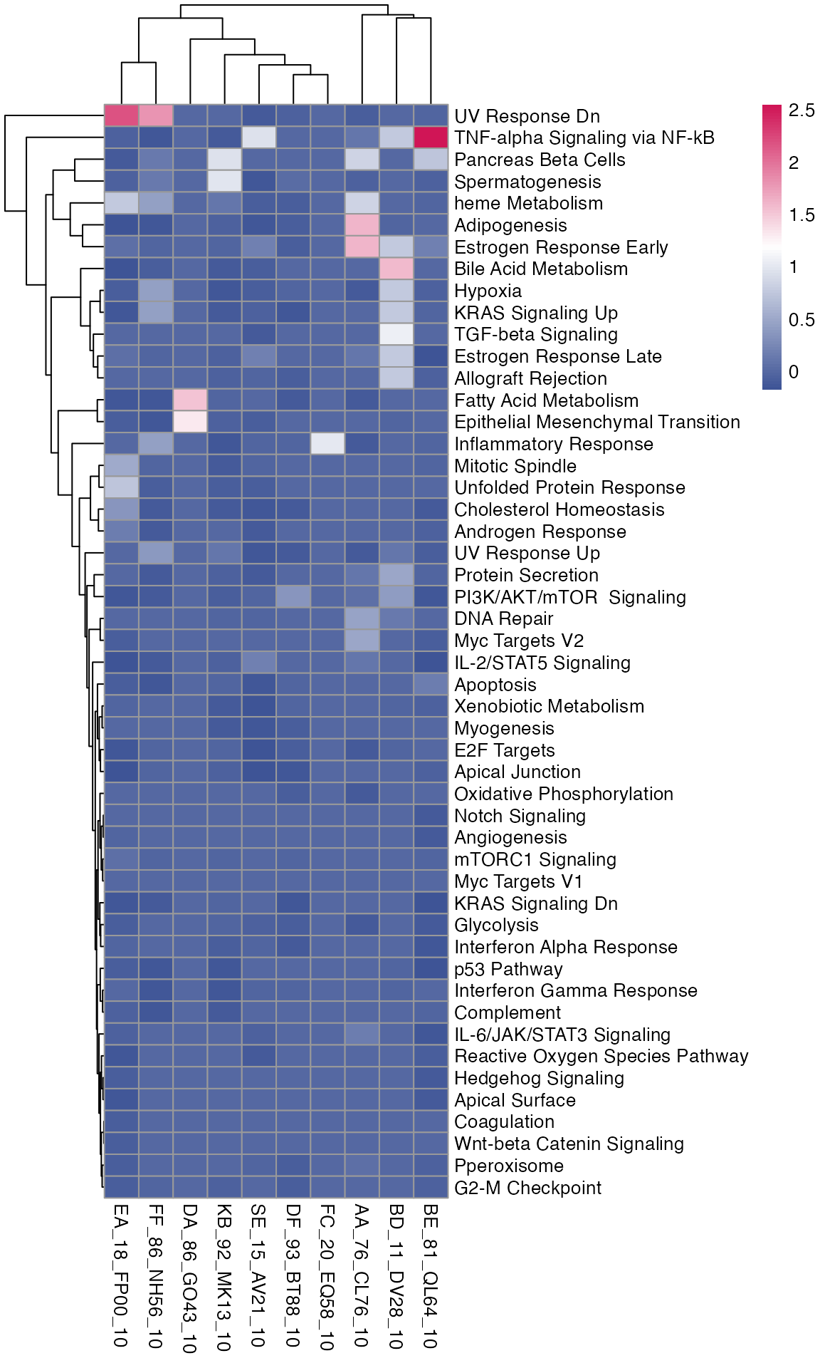

Benchmark

Selecting robust DMSO controls

We noticed that DRUGseq authors implemented a permutation strategy to identify robust DMSO wells in their analytics pipeline. We agree that robust control selection is critical for comparative benchmarking. The Novartis DRUGseq workflow selects DMSO controls via a 500-permutation procedure that retains wells minimising spurious DMSO–DMSO differentially expressed genes. To make this step practical for routine QC and for researchers with fewer DMSO wells, we implemented an alternative method in our macpie package select_robust_controls function that uses correlation-based selection of control wells.

This function ranks control wells based on their average Fisher-z-transformed correlation coefficients to all other control wells, selecting those with the highest average correlation scores as the ‘robust’ controls.

The DRUGseq data contains three replicate plates with 48 DMSO controls (CB-43-EP73). We applied our select_robust_controls function to these DMSO wells. It filters genes, normalises with TMMwsp, computes log-CPM, and ranks wells by mean Fisher-z–transformed correlation to all other replicate wells. The top 5 wells with the highest transformed correlation were then compared to DRUGseq results.

We benchmark the performance of macpie’s select_robust_controls function on DRUGseq data to select robust DMSO controls from three replicate plates.

DRUGseq: 6 robust DMSO wells

First we load the file of robust DMSO control wells identified by the DRUGseq authors in their github repo.

Here, we show the robust DMSO wells for batch 24, which contains the three plates we are interested in (VH02012942, VH02012944, VH02012956).

These 6 robust DMSO wells are used as the benchmark standard to compare with macpie selected robust DMSO wells.

robust_DMSO_DRUGseq <- read.csv(paste0(dir, "DRUGseqData/robust_RC_ReferenceControl_DMSO_wells.txt"), sep="")
robust_DMSO_DRUGseq %>% filter(batch_id==24) %>% select(batch_id, plate_barcode, well_id)
#>   batch_id plate_barcode well_id
#> 1       24    VH02012942     I23
#> 2       24    VH02012942     M23
#> 3       24    VH02012944     D23
#> 4       24    VH02012944     H23
#> 5       24    VH02012956     I23
#> 6       24    VH02012956     J23

As from their results of robust DMSO controls, these are the robust DMSO wells for batch 24:

VH02012942: I23, M23

VH02012944: D23, H23

VH02012956: I23, J23

macpie: select robust DMSO wells

Now we will use a function select_robust_controls to identify robust DMSO controls from batch 24.

This function:

applies CPM filtering,
performs TMMwsp normalisation and computes log-CPM,
ranks wells by their mean Fisher-z–transformed sample–sample correlation to all other wells (Pearson or Spearman)
selects the top n wells (user-defined) as robust controls.

mac_filtered <- readRDS(paste0(dir, "/DRUGseqData/macpie_filtered_batch24.Rds"))
mac_filtered$combined_id <- str_replace_all(mac_filtered$combined_id, "-","_")

Now we will apply the select_robust_controls function to each of the three plates in batch 24 to identify robust DMSO controls.

This function generates three plots:

Boxplot of log2-CPM (TMMwsp)
Sample–sample correlation (Pearson, log2-CPM)
Sample–sample correlation (Spearman, log2-CPM)

These plots help to visualize the distribution of gene expression and the correlation between samples, aiding in the assessment of DMSO control quality.

#to use lapply on three plates
plates <- c("VH02012942", "VH02012944", "VH02012956")
results <- lapply(plates, function(plate) {
  select_robust_controls(
    mac_filtered,
    samples = "CB_43_EP73_0",
    orig_ident  = plate,
    cpm_filter  = 1,
    min_samps   = 8,
    corr_method = "spearman",
    top_n       = 5,
    make_plots  = FALSE
  )
})

names(results) <- plates

As make_plots = FALSE in the above function, we can now visualise the plots for each plate separately. If you set make_plots = TRUE, the function will automatically generate the plots for you.

Plate VH02012942

pheatmap::pheatmap(results$VH02012942$cor_pearson,
  main = "Sample-sample Pearson correlation (log2-CPM)", 
  fontsize_row = 8, fontsize_col = 8)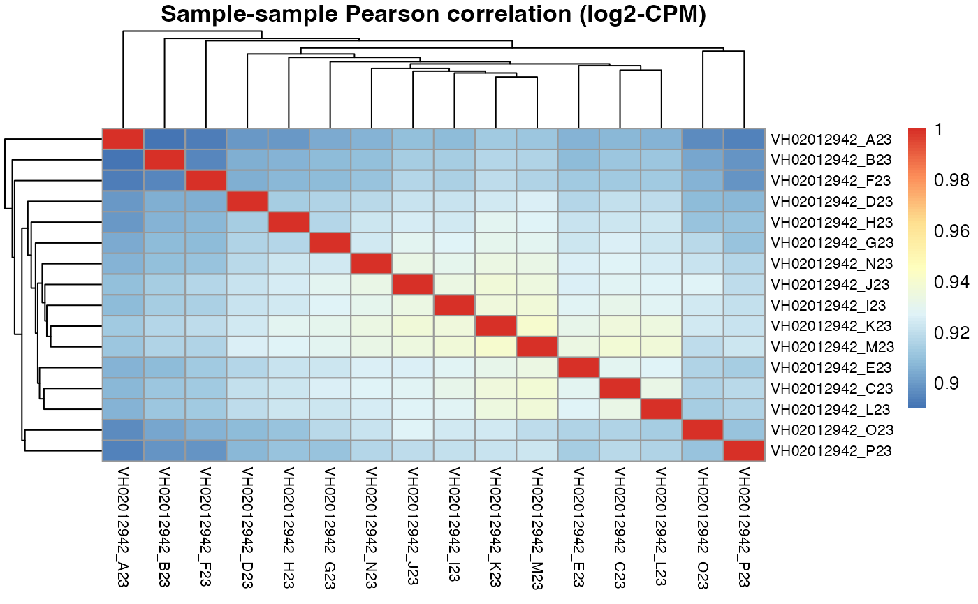

pheatmap::pheatmap(results$VH02012942$cor_spearman,
  main = "Sample-sample Spearman correlation (log2-CPM)", 
  fontsize_row = 8, fontsize_col = 8)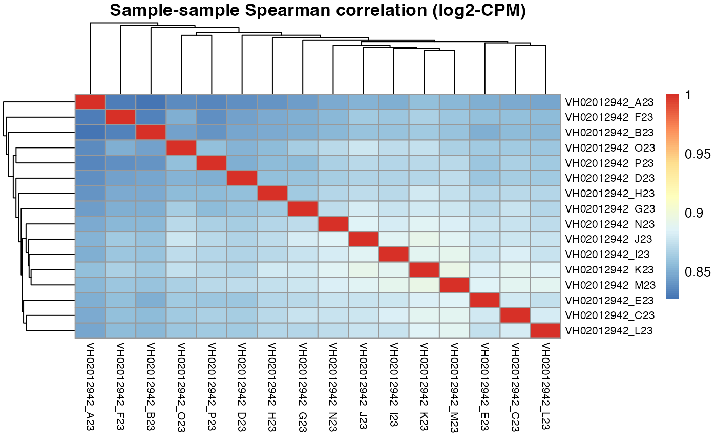

Apart from correlation heatmaps, the function also returns a ranking of wells by their mean correlation to all other wells.

results$VH02012942$scores_mean_to_others
#> VH02012942_K23 VH02012942_M23 VH02012942_J23 VH02012942_I23 VH02012942_C23 
#>          0.878          0.877          0.875          0.874          0.872 
#> VH02012942_N23 VH02012942_L23 VH02012942_E23 VH02012942_G23 VH02012942_H23 
#>          0.870          0.869          0.869          0.866          0.863 
#> VH02012942_O23 VH02012942_D23 VH02012942_P23 VH02012942_F23 VH02012942_B23 
#>          0.860          0.858          0.858          0.851          0.849 
#> VH02012942_A23 
#>          0.843

Finally, it returns the top N wells as robust DMSO controls.

results$VH02012942$topN
#> VH02012942_K23 VH02012942_M23 VH02012942_J23 VH02012942_I23 VH02012942_C23 
#>          0.878          0.877          0.875          0.874          0.872

Now we can see for plate VH02012942, the 2 of top 5 DMSO wells selected by macpie are I23 and J23, which are exactly the same as the robust DMSO wells identified by the DRUGseq authors.

Let’s repeat the same process for the other two plates in batch 24.

Plate VH02012944

pheatmap::pheatmap(results$VH02012944$cor_pearson,
  main = "Sample-sample Pearson correlation (log2-CPM)", 
  fontsize_row = 8, fontsize_col = 8)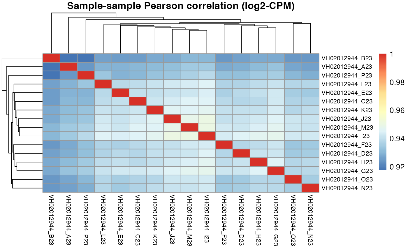

pheatmap::pheatmap(results$VH02012944$cor_spearman,
  main = "Sample-sample Spearman correlation (log2-CPM)", 
  fontsize_row = 8, fontsize_col = 8)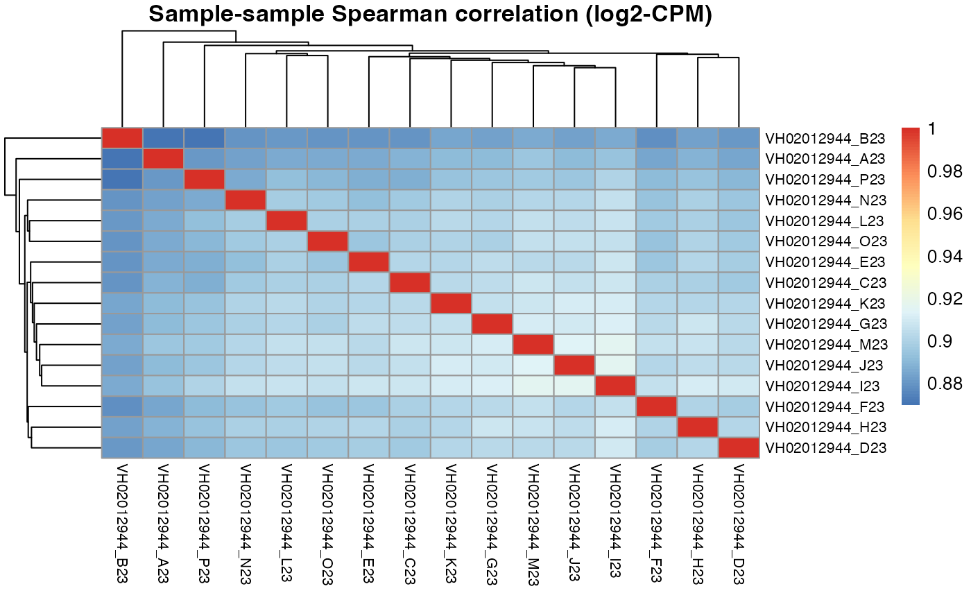

Apart from correlation heatmaps, the function also returns a ranking of wells by their mean correlation to all other wells.

results$VH02012944$scores_mean_to_others
#> VH02012944_I23 VH02012944_M23 VH02012944_J23 VH02012944_G23 VH02012944_K23 
#>          0.906          0.904          0.903          0.902          0.901 
#> VH02012944_H23 VH02012944_C23 VH02012944_L23 VH02012944_E23 VH02012944_D23 
#>          0.900          0.899          0.898          0.897          0.897 
#> VH02012944_O23 VH02012944_F23 VH02012944_N23 VH02012944_P23 VH02012944_A23 
#>          0.897          0.897          0.895          0.890          0.887 
#> VH02012944_B23 
#>          0.880

Finally, it returns the top N wells as robust DMSO controls.

results$VH02012944$topN
#> VH02012944_I23 VH02012944_M23 VH02012944_J23 VH02012944_G23 VH02012944_K23 
#>          0.906          0.904          0.903          0.902          0.901

For plate VH02012944, the DRUGseq selected D23 and H23 DMSO wells are not in our top 5. However, H23 is ranked 6th by macpie, which is very close to the top 5.

Plate VH02012956

pheatmap::pheatmap(results$VH02012956$cor_pearson,
  main = "Sample-sample Pearson correlation (log2-CPM)", 
  fontsize_row = 8, fontsize_col = 8)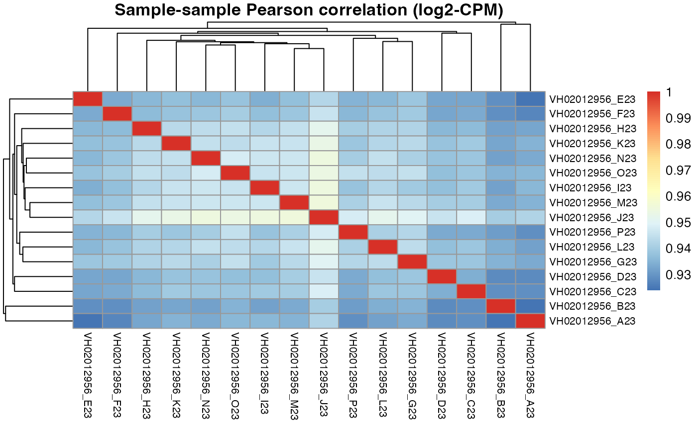

pheatmap::pheatmap(results$VH02012956$cor_spearman,
  main = "Sample-sample Spearman correlation (log2-CPM)", 
  fontsize_row = 8, fontsize_col = 8)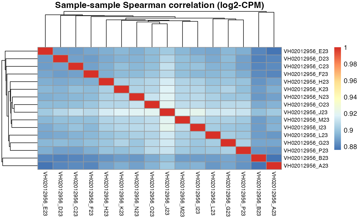

Apart from correlation heatmaps, the function also returns a ranking of wells by their mean correlation to all other wells.

results$VH02012956$scores_mean_to_others
#> VH02012956_J23 VH02012956_O23 VH02012956_M23 VH02012956_I23 VH02012956_K23 
#>          0.912          0.904          0.902          0.902          0.901 
#> VH02012956_N23 VH02012956_G23 VH02012956_H23 VH02012956_L23 VH02012956_P23 
#>          0.901          0.900          0.899          0.899          0.897 
#> VH02012956_F23 VH02012956_C23 VH02012956_D23 VH02012956_E23 VH02012956_A23 
#>          0.894          0.893          0.892          0.891          0.888 
#> VH02012956_B23 
#>          0.886

Finally, it returns the top N wells as robust DMSO controls.

results$VH02012942$topN
#> VH02012942_K23 VH02012942_M23 VH02012942_J23 VH02012942_I23 VH02012942_C23 
#>          0.878          0.877          0.875          0.874          0.872

For plate VH02012956, the DRUGseq selected I23 and J23 DMSO wells are exactly the same as our top DMSO wells selected by macpie.

Summary

To summarise the performance of macpie in selecting robust DMSO wells, we compare our selected top 5 DMSO wells with the DRUGseq authors’ selected robust DMSO wells for each plate in batch 24.

# DRUG-seq authors' robust DMSO wells (batch 24)
expected_df <- as_tibble(data.frame(
  plate = c("VH02012942", "VH02012942", "VH02012944", "VH02012944", "VH02012956", "VH02012956"),
  well  = c("I23", "M23", "D23", "H23", "I23", "J23"),
  source = "expected"))


# Helper: extract topN wells (names are like "VH02012942_I23")
extract_top_wells <- function(res_per_plate) {
  tibble(sample = names(res_per_plate$topN),
         score  = as.numeric(res_per_plate$topN)) |>
    mutate(
      plate = sub("_.*$", "", sample),
      well  = sub("^.*_", "", sample),
      rank  = row_number()
    ) |>
    select(plate, well, rank, score)
}

top_df <- map_df(names(results), ~{
  extract_top_wells(results[[.x]])
})


matched_df <- expected_df |>
  left_join(top_df, by = c("plate", "well")) |>
  mutate(found = !is.na(rank))


plate_summary <- matched_df |>
  group_by(plate) |>
  summarise(
    expected = n(),
    recovered = sum(found),
    recovery_rate = recovered / expected
  )

plate_summary
#> # A tibble: 3 × 4
#>   plate      expected recovered recovery_rate
#>   <chr>         <int>     <int>         <dbl>
#> 1 VH02012942        2         2             1
#> 2 VH02012944        2         0             0
#> 3 VH02012956        2         2             1

overall <- summarise(plate_summary,
                     total_expected = sum(expected),
                     total_recovered = sum(recovered),
                     overall_rate = total_recovered / total_expected)
overall
#> # A tibble: 1 × 3
#>   total_expected total_recovered overall_rate
#>            <int>           <int>        <dbl>
#> 1              6               4        0.667

ggplot(plate_summary, aes(x = plate, y = recovered, fill = plate)) +
  geom_col(width = 0.6, show.legend = FALSE) +
  geom_text(aes(label = sprintf("%d / %d (%.0f%%)",
                                recovered, expected, 100*recovery_rate)),
            vjust = -0.6) +
  ylim(0, max(plate_summary$expected) + 0.8) +
  labs(title = "Recovered DRUG-seq robust DMSO wells by plate",
       x = "Plate", y = "Recovered wells") +
  theme_classic()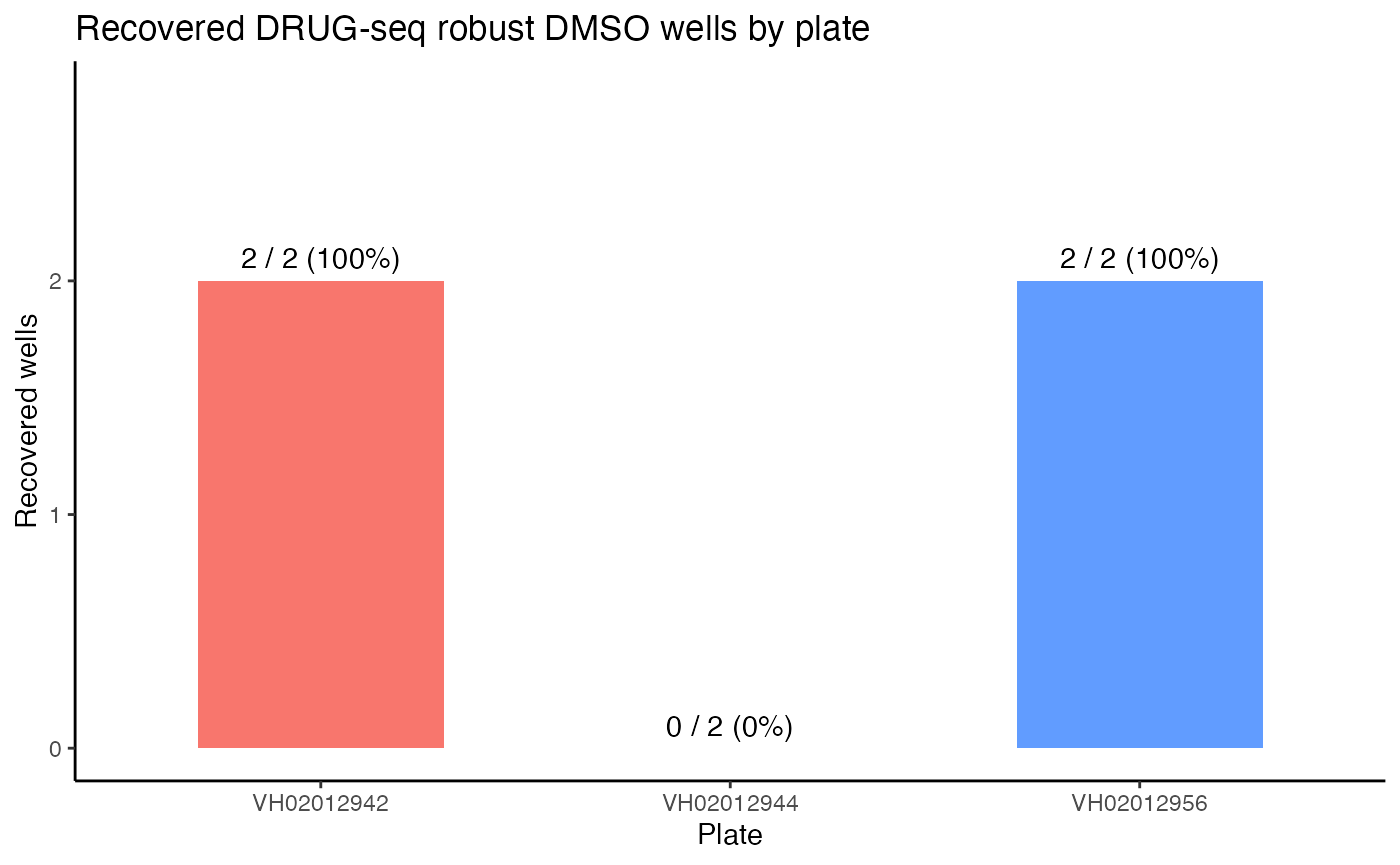

In summary, for the three plates in batch 24, macpie successfully identified 4 out of 6 robust DMSO wells (with ~66.7% overall recovery rate) that were also selected by the DRUGseq authors. Only for plate VH02012944, one of the DRUGseq selected DMSO wells (D23) was not in our top 5, but the other well (H23) was ranked 6th by macpie, which is very close to the top 5. This demonstrates that macpie is effective in selecting high-quality DMSO controls for downstream analysis without running permutation tests, making it a computationally efficient choice.

This function runs for each plate, it does not take into account any batches or plates. If it’s a cross-plates design, it is recommended to either compute within-plate or remove plate effects (e.g. using ComBat, limma removeBatchEffect functions) first.

DEG concordance

Now we compare macpie implementations of limma-voom, edgeR, DEseq2 and limma-trend against DRUGseq limma-trend result on the FF_86_NH56 (10uM) vs DMSO control from batch 24. We evaluated three control settings: (i) all DMSO wells (48 wells), (ii) top 15 DMSO selected by our correlation-based approach, and (iii) 6 DMSO wells identified by DRUGseq 500 permutation-based method.

We only focus on up-regulated genes in FF_86_NH56 (genes were called DEG if BH-adjusted p < 0.05 and log2FC > 0).

DRUGseq DEG results

For the purpose of this vignette, we only load the DRUGseq DEG results for FF_86_NH56 (10uM) vs DMSO control from batch 24.

batch24_de <- readRDS(paste0(dir,"DRUGseqData/DE_batch24.Rds"))
FF86_res <- batch24_de %>% filter(cmpd_sample_id=="FF-86-NH56")
ff86_res_toptable <- FF86_res[,13:18]
ff86_res_toptable <- ff86_res_toptable %>% 
  separate(gene.ID, into = c("gene", "chrom"), sep = ",") %>%
  select(-chrom) %>% mutate(combined_id ="FF_86_NH56_10") %>%
  rename(log2FC=logFC, p_value_adj = adj.P.Val)

plot_volcano(ff86_res_toptable, max.overlaps =3)
#> Warning: ggrepel: 4344 unlabeled data points (too many overlaps). Consider
#> increasing max.overlaps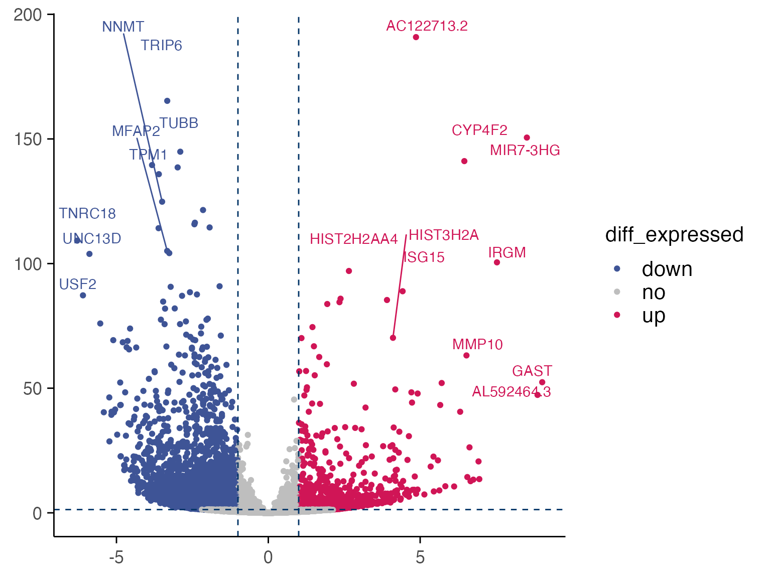

ff86_res_toptable %>% filter(p_value_adj <0.05 & log2FC >0) %>% nrow()
#> [1] 1423

drugseq_deg <- ff86_res_toptable %>% filter(p_value_adj <0.05 & log2FC >0) %>% select(gene) %>% pull()

There are 1423 up-regulated DEGs identified by DRUGseq limma-trend method for FF_86_NH56 (10uM) vs DMSO control from batch 24.

macpie DEG results with all DMSO wells

Load filered data

mac_filtered <- readRDS(paste0(dir, "/DRUGseqData/macpie_filtered_batch24.Rds"))
mac_filtered$combined_id <- str_replace_all(mac_filtered$combined_id, "-","_")

Differential gene expression

methods <- c("limma_voom", "DESeq2", "edgeR", "limma_trend")

methods_res <- lapply(methods, function(m){
  
  message("\n","Processing method: ", m,"\n") 
  # m<-"limma_voom"
  treatment_samples <- "FF_86_NH56_10"
  control_samples <- "CB_43_EP73_0"
  subset <- mac_filtered%>%filter(combined_id%in%c(treatment_samples,control_samples))

  batch <- subset$orig.ident


  top_table <- compute_single_de(subset, treatment_samples, control_samples, method =  m, batch = batch)
  
  # plot(plot_volcano(top_table, max.overlaps = 5))
  alldmso_degs <- top_table %>% filter(p_value_adj <0.05 & log2FC>0) %>% select(gene) %>% pull()
  length(intersect(alldmso_degs, drugseq_deg))
  
  top_table <- top_table %>%
    arrange(p_value_adj, desc(log2FC)) %>%
    mutate(gene = factor(gene, levels = unique(gene)))
  # add a column if there are in the intersect(alldmso_degs, drugseq_deg)
  top_table <- top_table %>%
    mutate(in_drugseq_deg = ifelse(gene %in% intersect(alldmso_degs, drugseq_deg), "yes", "no"))

  # label a few top overlapping genes
  lab_genes <- top_table[top_table$in_drugseq_deg=="yes", ] |>
    dplyr::arrange(p_value_adj, dplyr::desc(log2FC)) 
  
  volcano_overlap <- ggplot(top_table, aes(x = log2FC, y = -log10(p_value_adj), color = in_drugseq_deg)) +
    geom_point(alpha = 0.6, size = 1.2) +
    geom_text_repel(data = lab_genes, aes(label = gene), size = 3, max.overlaps = 50) +
    scale_color_manual(values = c("no"="#bdbdbd","yes"="#2b8cbe"))+
    theme_classic()
  
  
  #return 
  result_list <- list(top_table = top_table,
                      num_degs_macpie = length(alldmso_degs),
                      n_overlap = length(intersect(alldmso_degs, drugseq_deg)),
                      volcano_plot = volcano_overlap)

  return(result_list)
  
})
#> 
#> Processing method: limma_voom
#> 
#> Processing method: DESeq2
#> converting counts to integer mode
#> estimating size factors
#> estimating dispersions
#> gene-wise dispersion estimates
#> mean-dispersion relationship
#> -- note: fitType='parametric', but the dispersion trend was not well captured by the
#>    function: y = a/x + b, and a local regression fit was automatically substituted.
#>    specify fitType='local' or 'mean' to avoid this message next time.
#> final dispersion estimates
#> fitting model and testing
#> -- replacing outliers and refitting for 1196 genes
#> -- DESeq argument 'minReplicatesForReplace' = 7 
#> -- original counts are preserved in counts(dds)
#> estimating dispersions
#> fitting model and testing
#> 
#> Processing method: edgeR
#> 
#> Processing method: limma_trend

names(methods_res) <- methods

Summary table

#get a table to show number of DEGs and number of overlapping genes with DRUGseq for each method
deg_summary <- map_df(methods_res, function(x) {
  data.frame(
    num_degs_macpie = x$num_degs_macpie,
    n_overlap = x$n_overlap,
    num_degs_DRUGseq = length(drugseq_deg)
  )
}, .id = paste0("macpie_methods"))

deg_summary
#>   macpie_methods num_degs_macpie n_overlap num_degs_DRUGseq
#> 1     limma_voom            5597       890             1423
#> 2         DESeq2            2188       817             1423
#> 3          edgeR            2340       719             1423
#> 4    limma_trend            3047       666             1423

Overlapping volcano plot

methods_res$limma_voom$volcano_plot
#> Warning: ggrepel: 862 unlabeled data points (too many overlaps). Consider
#> increasing max.overlaps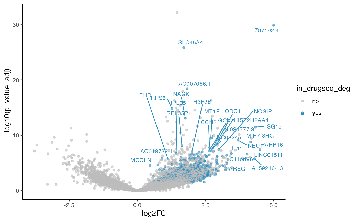

methods_res$DESeq2$volcano_plot
#> Warning: Removed 3480 rows containing missing values or values outside the scale range
#> (`geom_point()`).
#> Warning: ggrepel: 779 unlabeled data points (too many overlaps). Consider
#> increasing max.overlaps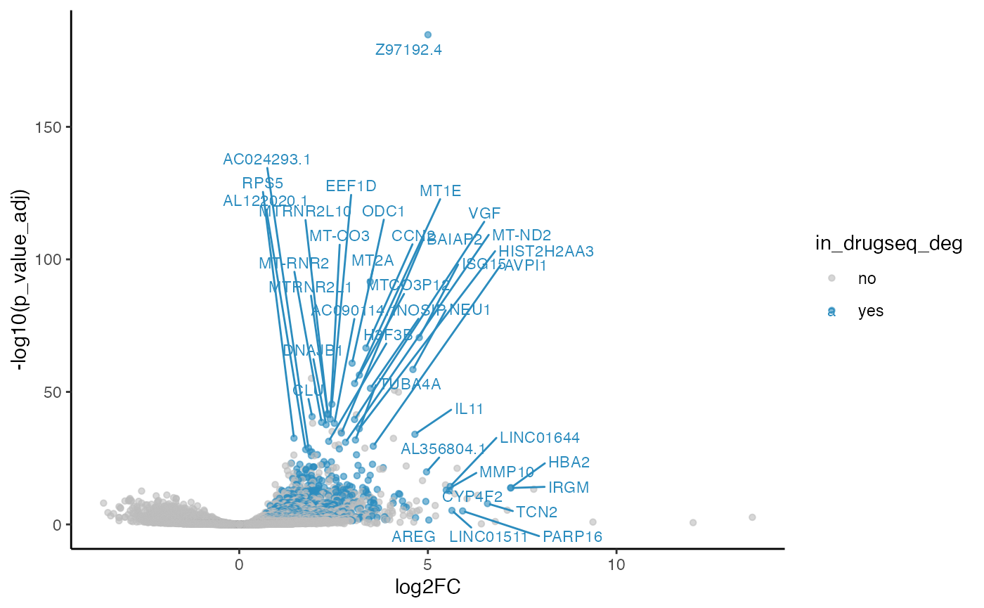

methods_res$edgeR$volcano_plot
#> Warning: ggrepel: 652 unlabeled data points (too many overlaps). Consider
#> increasing max.overlaps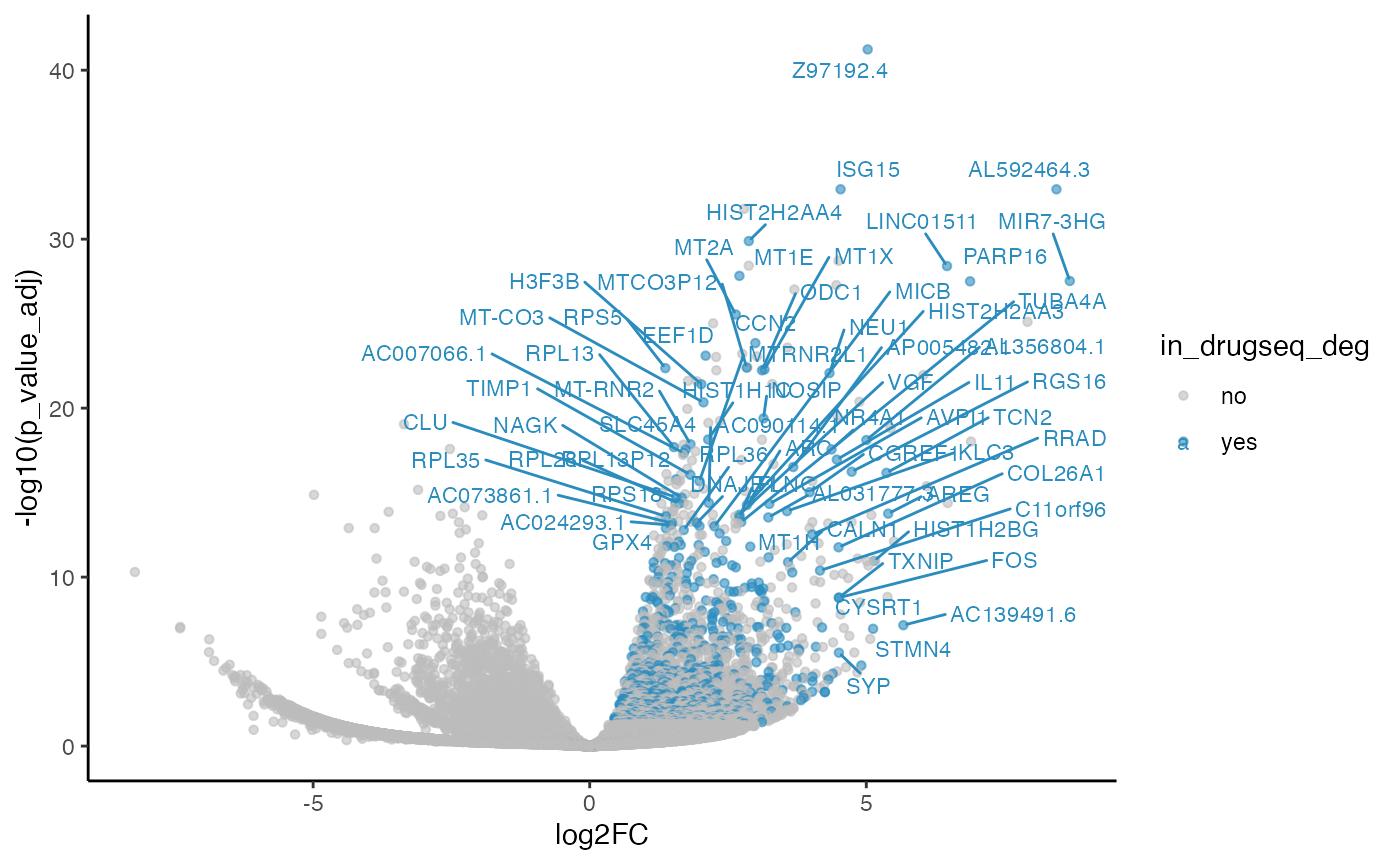

methods_res$limma_trend$volcano_plot
#> Warning: ggrepel: 644 unlabeled data points (too many overlaps). Consider
#> increasing max.overlaps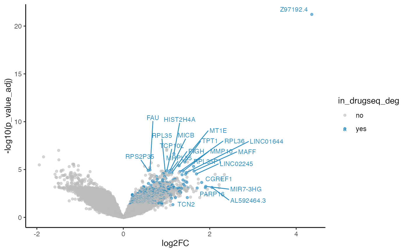

macpie DEG results with 15 robust DMSO wells

From our select_robust_controls function above, we identified the following top 15 DMSO wells from three plates in batch 24 using select_robust_controls:

batch24 <- readRDS(paste0(dir,"DRUGseqData/Exp_batch24.Rds"))
names(batch24)
#> [1] "VH02012956" "VH02012942" "VH02012944"

#make a combined metadata for three plates
batch24_metadata <- batch24 %>% 
  map_dfr(~ {
    .x$Annotation %>%
      mutate(
        Plate_ID        = plate_barcode,
        Well_ID         = well_id,
        Barcode         = paste0(plate_barcode, "_", well_index),
        Row             = LETTERS[row],
        Column          = as.integer(col),
        Species         = "human",
        Cell_type       = "U2OS",
        Model_type      = "2D_adherent",
        Time            = as.factor(hours_post_treatment),
        Unit            = "h",
        Treatment_1     = cmpd_sample_id,
        Concentration_1 = as.numeric(concentration),
        Unit_1          = unit,
        Sample_type     = if_else(well_type == "SA" & col == 24,
                                  "Positive Control",
                                  well_type)
      )
  })


batch24_metadata <- batch24_metadata%>%select(-c(batch_id, plate_barcode,plate_index, well_id,
                                                 well_index, col, row, biosample_id, external_biosample_id,
                                                 cmpd_sample_id, well_type, cell_line_name, cell_line_ncn, concentration, unit, hours_post_treatment, Sample))

# create a combined UMI matrix for 3 plates
batch24_counts <- batch24 %>%
  map(~ {
    .x$UMI.counts %>%
      as.data.frame() %>% 
      rownames_to_column("gene_id") %>%
      separate(col = gene_id, into = c("gene_name", "chrom"), sep = ",") %>%
      mutate(gene_name = make.unique(gene_name)) %>%
      select(-chrom) %>%
      tibble::column_to_rownames(var = "gene_name") %>%
      as.matrix()
  })

binded_counts <- do.call(cbind, batch24_counts)

as_mac <- CreateSeuratObject(counts = binded_counts, 
  min.cells = 1, 
  min.features = 1)
#> Warning: Feature names cannot have underscores ('_'), replacing with dashes
#> ('-')
#> Warning: Data is of class matrix. Coercing to dgCMatrix.

as_mac<- as_mac%>% inner_join(batch24_metadata, by = c(".cell"="Barcode"))


as_mac$combined_id <- paste0(as_mac$Treatment_1,"_", as_mac$Concentration_1)

badDMSO <- as_mac@meta.data %>% filter(Treatment_1 == "CB-43-EP73") %>% 
 filter((Plate_ID == "VH02012942" & !(Well_ID %in% c("I23", "M23", "K23", "J23","C23"))) |
        (Plate_ID == "VH02012944" & !(Well_ID %in% c("I23", "M23", "J23", "G23", "K23")))|
        (Plate_ID == "VH02012956" & !  (Well_ID %in% c("I23", "J23", "O23","M23","K23"))))



keep_wells <- setdiff(rownames(as_mac@meta.data), rownames(badDMSO))


mac_badDSMOremoved <- as_mac[,keep_wells]

mac_badDSMOremoved$combined_id <- str_replace_all(mac_badDSMOremoved$combined_id, "-","_")

min_sample_num <- min(table(mac_badDSMOremoved$combined_id))
mac_badDSMOremoved <- filter_genes_by_expression(mac_badDSMOremoved,
                                           group_by = "combined_id", min_counts =10,
                                           min_samples = min_sample_num)

Differential gene expression

methods <- c("limma_voom", "DESeq2", "edgeR", "limma_trend")

five_dmso_methods_res <- lapply(methods, function(m){
  message("Processing method: ", m) 
  # m<-"limma_voom"
  treatment_samples <- "FF_86_NH56_10"
  control_samples <- "CB_43_EP73_0"
  subset <- mac_badDSMOremoved%>%filter(combined_id%in%c(treatment_samples,control_samples))

  batch <- subset$orig.ident

  badDMSO_out_top_table <- compute_single_de(subset, treatment_samples, control_samples, method =  m, batch = batch)

 
  # plot(plot_volcano(top_table, max.overlaps = 5))
  badDMSO_out_degs <- badDMSO_out_top_table %>% filter(p_value_adj <0.05 & log2FC>0) %>% select(gene) %>% pull()
  length(intersect(badDMSO_out_degs, drugseq_deg))
  
  badDMSO_out_top_table <- badDMSO_out_top_table %>%
    arrange(p_value_adj, desc(log2FC)) %>%
    mutate(gene = factor(gene, levels = unique(gene)))
  # add a column if there are in the intersect(alldmso_degs, drugseq_deg)
  badDMSO_out_top_table <- badDMSO_out_top_table %>%
    mutate(in_drugseq_deg = ifelse(gene %in% intersect(badDMSO_out_degs, drugseq_deg), "yes", "no"))
  
  # label a few top overlapping genes
  lab_genes <- badDMSO_out_top_table[badDMSO_out_top_table$in_drugseq_deg=="yes", ] |>
    dplyr::arrange(p_value_adj, dplyr::desc(log2FC)) 
  
  volcano_overlap <- ggplot(badDMSO_out_top_table, aes(x = log2FC, y = -log10(p_value_adj), color = in_drugseq_deg)) +
    geom_point(alpha = 0.6, size = 1.2) +
    geom_text_repel(data = lab_genes, aes(label = gene), size = 3, max.overlaps = 10) +
    scale_color_manual(values = c("no"="#bdbdbd","yes"="#2b8cbe"))+
    theme_classic()

  #return 
  result_list <- list(top_table = badDMSO_out_top_table,
                      num_degs_macpie = length(badDMSO_out_degs),
                      n_overlap = length(intersect(badDMSO_out_degs, drugseq_deg)),
                      volcano_plot = volcano_overlap)
  return(result_list)
  
})
#> Processing method: limma_voom
#> Processing method: DESeq2
#> converting counts to integer mode
#> estimating size factors
#> estimating dispersions
#> gene-wise dispersion estimates
#> mean-dispersion relationship
#> final dispersion estimates
#> fitting model and testing
#> Processing method: edgeR
#> Processing method: limma_trend

names(five_dmso_methods_res) <- methods

Summary table

#get a table to show number of DEGs and number of overlapping genes with DRUGseq for each method
deg_summary <- map_df(five_dmso_methods_res, function(x) {
  data.frame(
    num_degs_macpie = x$num_degs_macpie,
    n_overlap = x$n_overlap,
    num_degs_DRUGseq = length(drugseq_deg)
  )
}, .id = paste0("macpie_methods"))

deg_summary
#>   macpie_methods num_degs_macpie n_overlap num_degs_DRUGseq
#> 1     limma_voom            3456       592             1423
#> 2         DESeq2            1107       549             1423
#> 3          edgeR            2185       690             1423
#> 4    limma_trend              60        15             1423

Overlapping volcano plot

five_dmso_methods_res$limma_voom$volcano_plot
#> Warning: ggrepel: 575 unlabeled data points (too many overlaps). Consider
#> increasing max.overlaps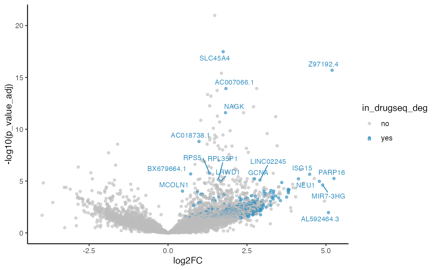

five_dmso_methods_res$DESeq2$volcano_plot
#> Warning: Removed 12331 rows containing missing values or values outside the scale range
#> (`geom_point()`).
#> Warning: ggrepel: 535 unlabeled data points (too many overlaps). Consider
#> increasing max.overlaps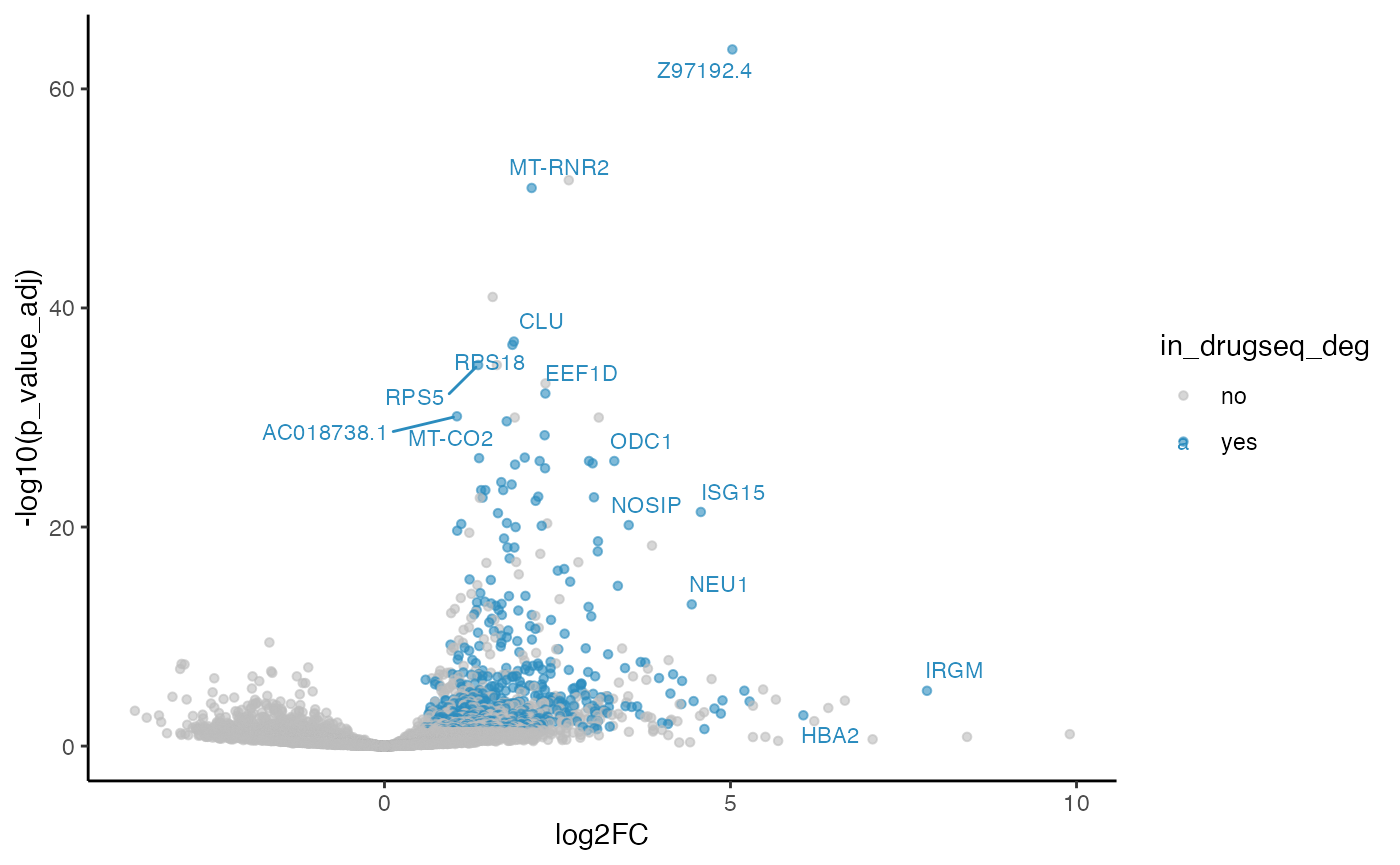

five_dmso_methods_res$edgeR$volcano_plot
#> Warning: ggrepel: 664 unlabeled data points (too many overlaps). Consider
#> increasing max.overlaps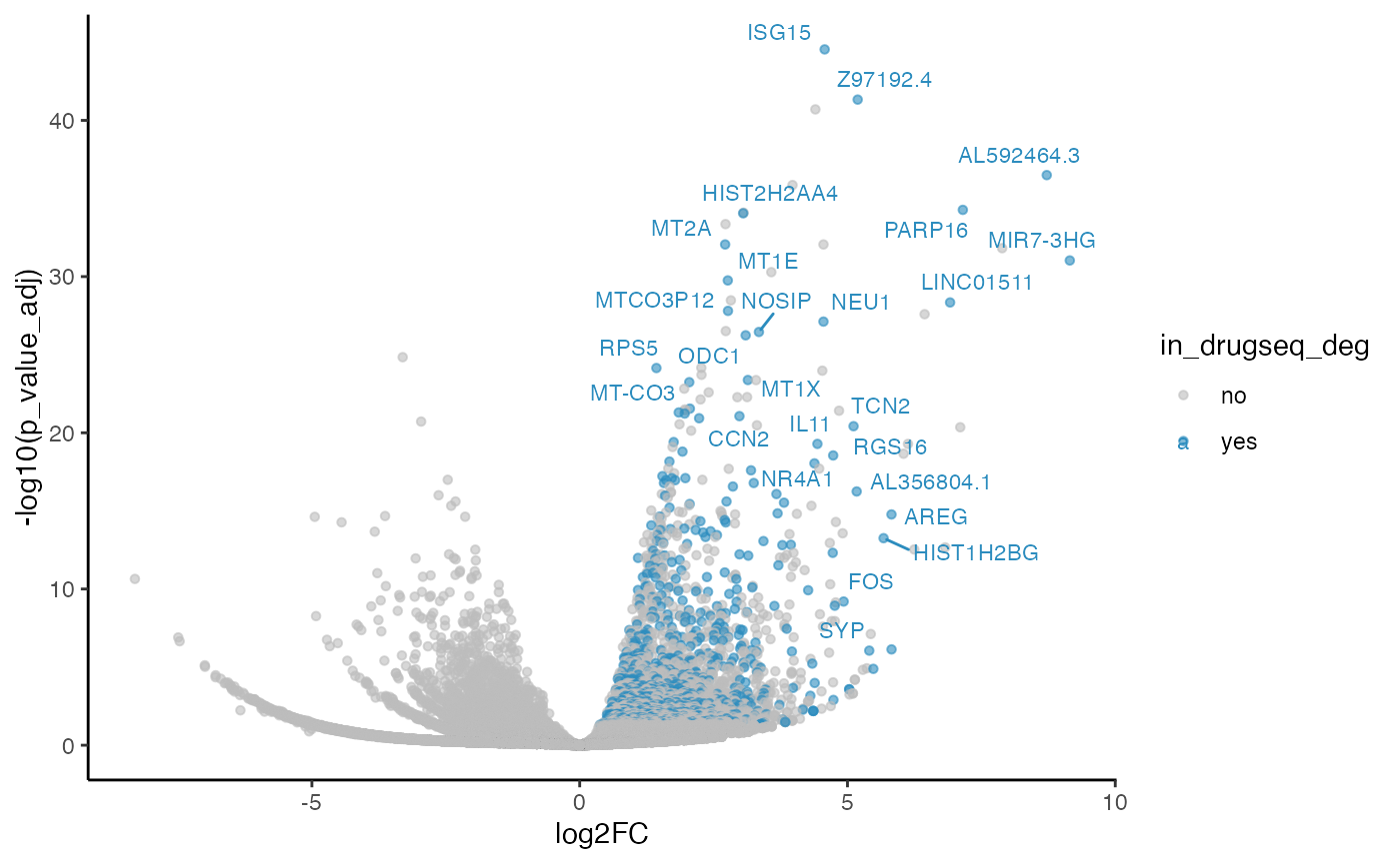

five_dmso_methods_res$limma_trend$volcano_plot
#> Warning: ggrepel: 11 unlabeled data points (too many overlaps). Consider
#> increasing max.overlaps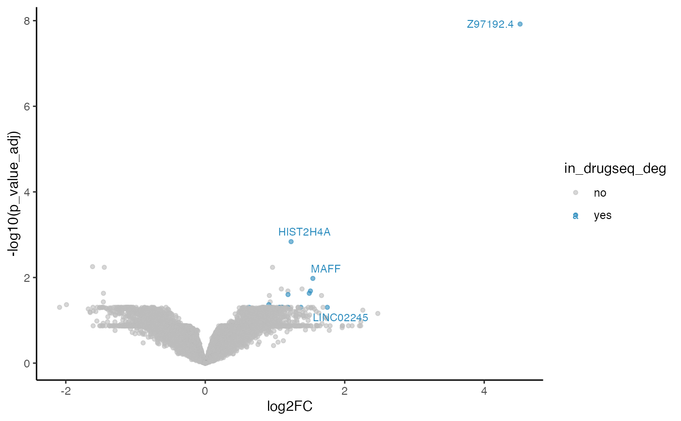

macpie DEG results with 6 robust DMSO wells from DRUGseq

From public DRUG-seq analysis pipeline, authors identified two reference controls: all DMSO wells and the ‘robust DMSO’ wells.

We know these robust DMSO wells for batch 24 from their published data:

VH02012942: I23, M23
VH02012944: D23, H23
VH02012956: I23, J23

batch24 <- readRDS(paste0(dir,"DRUGseqData/Exp_batch24.Rds"))
names(batch24)
#> [1] "VH02012956" "VH02012942" "VH02012944"

#make a combined metadata for three plates
batch24_metadata <- batch24 %>% 
  map_dfr(~ {
    .x$Annotation %>%
      mutate(
        Plate_ID        = plate_barcode,
        Well_ID         = well_id,
        Barcode         = paste0(plate_barcode, "_", well_index),
        Row             = LETTERS[row],
        Column          = as.integer(col),
        Species         = "human",
        Cell_type       = "U2OS",
        Model_type      = "2D_adherent",
        Time            = as.factor(hours_post_treatment),
        Unit            = "h",
        Treatment_1     = cmpd_sample_id,
        Concentration_1 = as.numeric(concentration),
        Unit_1          = unit,
        Sample_type     = if_else(well_type == "SA" & col == 24,
                                  "Positive Control",
                                  well_type)
      )
  })


batch24_metadata <- batch24_metadata%>%select(-c(batch_id, plate_barcode,plate_index, well_id,
                                                 well_index, col, row, biosample_id, external_biosample_id,
                                                 cmpd_sample_id, well_type, cell_line_name, cell_line_ncn, concentration, unit, hours_post_treatment, Sample))

# create a combined UMI matrix for 3 plates
batch24_counts <- batch24 %>%
  map(~ {
    .x$UMI.counts %>%
      as.data.frame() %>% 
      rownames_to_column("gene_id") %>%
      separate(col = gene_id, into = c("gene_name", "chrom"), sep = ",") %>%
      mutate(gene_name = make.unique(gene_name)) %>%
      select(-chrom) %>%
      tibble::column_to_rownames(var = "gene_name") %>%
      as.matrix()
  })

binded_counts <- do.call(cbind, batch24_counts)

as_mac <- CreateSeuratObject(counts = binded_counts, 
  min.cells = 1, 
  min.features = 1)
#> Warning: Feature names cannot have underscores ('_'), replacing with dashes
#> ('-')
#> Warning: Data is of class matrix. Coercing to dgCMatrix.

as_mac<- as_mac%>% inner_join(batch24_metadata, by = c(".cell"="Barcode"))


as_mac$combined_id <- paste0(as_mac$Treatment_1,"_", as_mac$Concentration_1)

badDMSO <- as_mac@meta.data %>% filter(Treatment_1 == "CB-43-EP73") %>% 
 filter((Plate_ID == "VH02012942" & !(Well_ID %in% c("I23", "M23"))) |
        (Plate_ID == "VH02012944" & !(Well_ID %in% c("D23", "H23")))|
        (Plate_ID == "VH02012956" & !  (Well_ID %in% c("I23", "J23"))))



keep_wells <- setdiff(rownames(as_mac@meta.data), rownames(badDMSO))


mac_badDSMOremoved <- as_mac[,keep_wells]

mac_badDSMOremoved$combined_id <- str_replace_all(mac_badDSMOremoved$combined_id, "-","_")

min_sample_num <- min(table(mac_badDSMOremoved$combined_id))
mac_badDSMOremoved <- filter_genes_by_expression(mac_badDSMOremoved,
                                           group_by = "combined_id", min_counts =10,
                                           min_samples = min_sample_num)

Differential gene expression

methods <- c("limma_voom", "DESeq2", "edgeR", "limma_trend")

robust_dmso_methods_res <- lapply(methods, function(m){
  message("Processing method: ", m) 
  # m<-"limma_voom"
  treatment_samples <- "FF_86_NH56_10"
  control_samples <- "CB_43_EP73_0"
  subset <- mac_badDSMOremoved%>%filter(combined_id%in%c(treatment_samples,control_samples))

  batch <- subset$orig.ident

  badDMSO_out_top_table <- compute_single_de(subset, treatment_samples, control_samples, method =  m, batch = batch)

  # plot(plot_volcano(top_table, max.overlaps = 5))
  badDMSO_out_degs <- badDMSO_out_top_table %>% filter(p_value_adj <0.05 & log2FC>0) %>% select(gene) %>% pull()
  length(intersect(badDMSO_out_degs, drugseq_deg))
  
  badDMSO_out_top_table <- badDMSO_out_top_table %>%
    arrange(p_value_adj, desc(log2FC)) %>%
    mutate(gene = factor(gene, levels = unique(gene)))
  # add a column if there are in the intersect(alldmso_degs, drugseq_deg)
  badDMSO_out_top_table <- badDMSO_out_top_table %>%
    mutate(in_drugseq_deg = ifelse(gene %in% intersect(badDMSO_out_degs, drugseq_deg), "yes", "no"))

  # label a few top overlapping genes
  lab_genes <- badDMSO_out_top_table[badDMSO_out_top_table$in_drugseq_deg=="yes", ] |>
    dplyr::arrange(p_value_adj, dplyr::desc(log2FC)) 
  
  volcano_overlap <- ggplot(badDMSO_out_top_table, aes(x = log2FC, y = -log10(p_value_adj), color = in_drugseq_deg)) +
    geom_point(alpha = 0.6, size = 1.2) +
    geom_text_repel(data = lab_genes, aes(label = gene), size = 3, max.overlaps = 10) +
    scale_color_manual(values = c("no"="#bdbdbd","yes"="#2b8cbe"))+
    theme_classic()
  
  #return 
  result_list <- list(top_table = badDMSO_out_top_table,
                      num_degs_macpie = length(badDMSO_out_degs),
                      n_overlap = length(intersect(badDMSO_out_degs, drugseq_deg)),
                      volcano_plot = volcano_overlap)
  return(result_list)
  
})
#> Processing method: limma_voom
#> Processing method: DESeq2
#> converting counts to integer mode
#> estimating size factors
#> estimating dispersions
#> gene-wise dispersion estimates
#> mean-dispersion relationship
#> final dispersion estimates
#> fitting model and testing
#> Processing method: edgeR
#> Processing method: limma_trend

names(robust_dmso_methods_res) <- methods

Summary table

#get a table to show number of DEGs and number of overlapping genes with DRUGseq for each method
deg_summary <- map_df(robust_dmso_methods_res, function(x) {
  data.frame(
    num_degs_macpie = x$num_degs_macpie,
    n_overlap = x$n_overlap,
    num_degs_DRUGseq = length(drugseq_deg)
  )
}, .id = paste0("macpie_methods"))

deg_summary
#>   macpie_methods num_degs_macpie n_overlap num_degs_DRUGseq
#> 1     limma_voom            1352       204             1423
#> 2         DESeq2              10         8             1423
#> 3          edgeR            1757       604             1423
#> 4    limma_trend               1         1             1423

Overlapping volcano plot

robust_dmso_methods_res$limma_voom$volcano_plot
#> Warning: ggrepel: 196 unlabeled data points (too many overlaps). Consider
#> increasing max.overlaps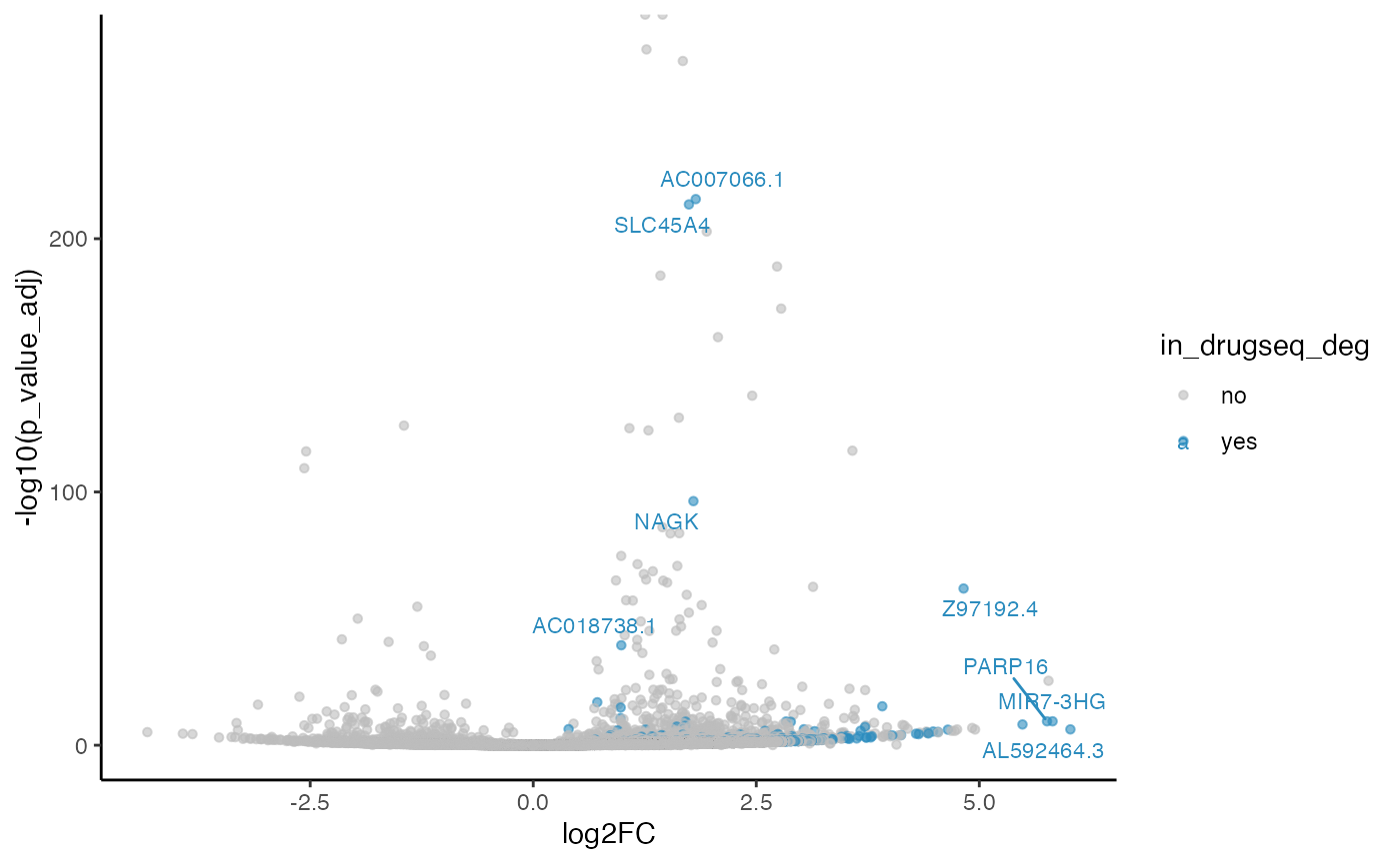

robust_dmso_methods_res$DESeq2$volcano_plot
#> Warning: Removed 19705 rows containing missing values or values outside the scale range
#> (`geom_point()`).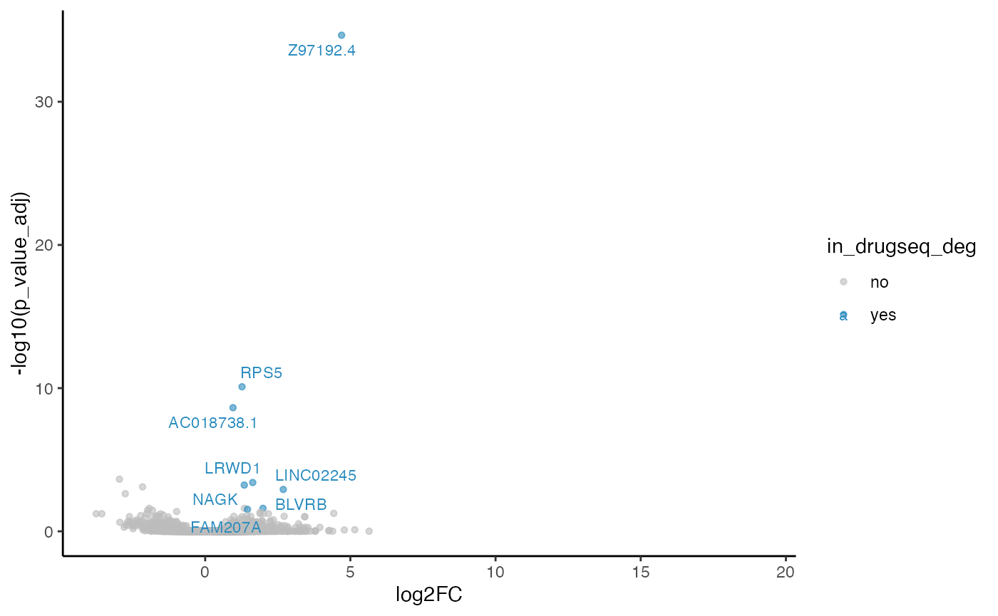

robust_dmso_methods_res$edgeR$volcano_plot
#> Warning: ggrepel: 583 unlabeled data points (too many overlaps). Consider
#> increasing max.overlaps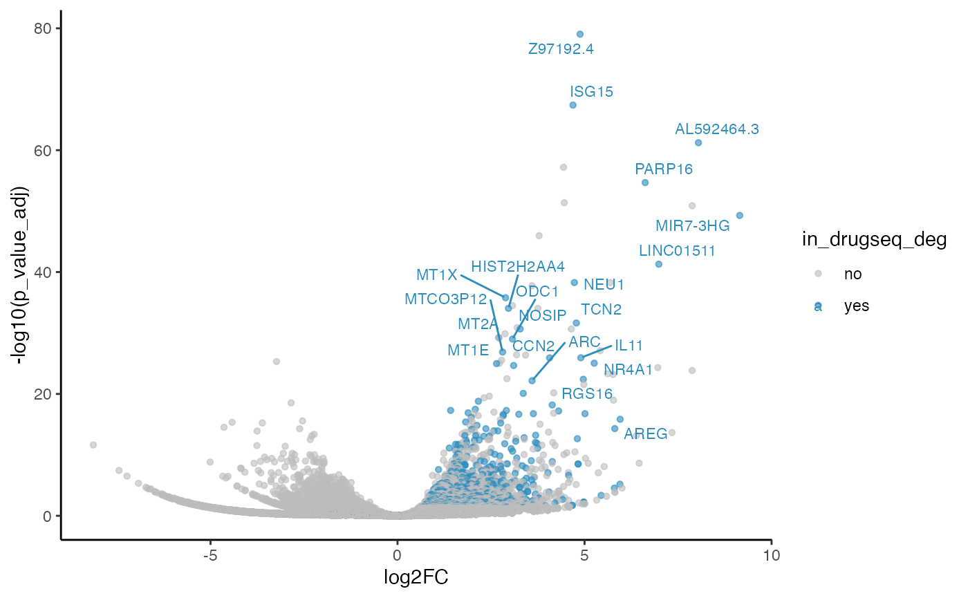

robust_dmso_methods_res$limma_trend$volcano_plot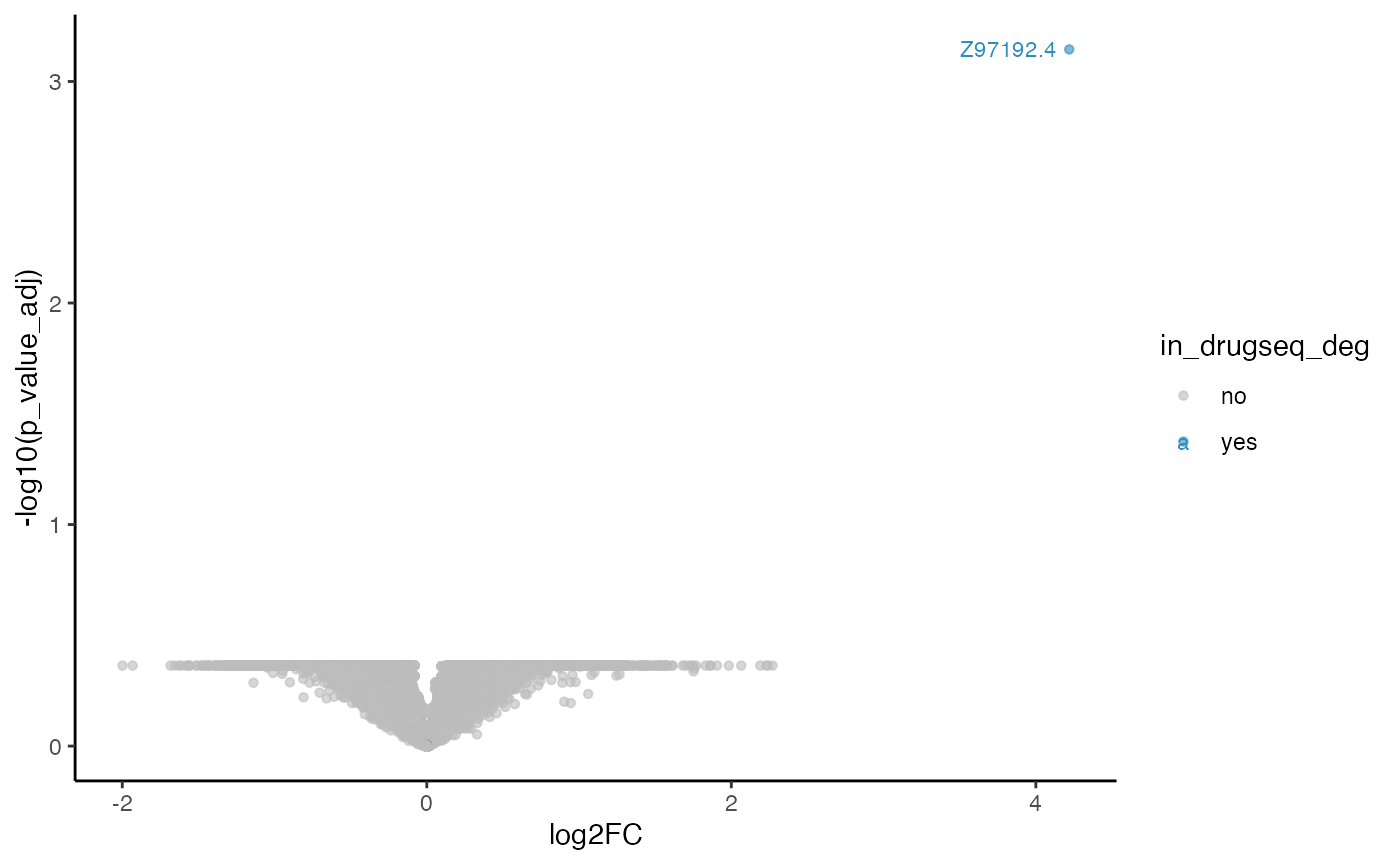

Summary of DEG concordance

To compare DEGs with different replicate numbers and different methods

methods <- c("limma_voom", "DESeq2", "edgeR", "limma_trend")

get_jaccard <- function(deg_set, drugseq_deg){
  intersection <- length(intersect(deg_set, drugseq_deg))
  union <- length(union(deg_set, drugseq_deg))
  jaccard_index <- intersection / union
  return(jaccard_index)
}

jaccard_index <- lapply(methods, function(m){
  # all dmso
  degs <- methods_res[[m]]$top_table %>% filter(p_value_adj <0.05 & log2FC>0) %>% select(gene) %>% pull()
  jaccard_all <- get_jaccard(degs, drugseq_deg)
  # five dmso
  degs <- five_dmso_methods_res[[m]]$top_table %>% filter(p_value_adj <0.05 & log2FC>0) %>% select(gene) %>% pull()
  jaccard_five <- get_jaccard(degs, drugseq_deg)
  # three dmso
  degs <- robust_dmso_methods_res[[m]]$top_table %>% filter(p_value_adj <0.05 & log2FC>0) %>% select(gene) %>% pull()
  jaccard_three <- get_jaccard(degs, drugseq_deg)
  jaccard_index <- data.frame(
    method = m,
    jaccard_all = jaccard_all,
    jaccard_five = jaccard_five,
    jaccard_three = jaccard_three
  )
  return(jaccard_index)
})

df <- as.data.frame(do.call(rbind, jaccard_index))
rownames(df) <- df$method
df <- df %>% select(-method)
colnames(df) <- c("All DMSO", "macpie: 15 DMSO", "DRUGseq: 6 DMSO")
pheatmap::pheatmap(df,
         cluster_rows = FALSE,
         cluster_cols = FALSE,
         display_numbers = TRUE,
         main = "Jaccard Index between macpie DEGs and DRUGseq DEGs")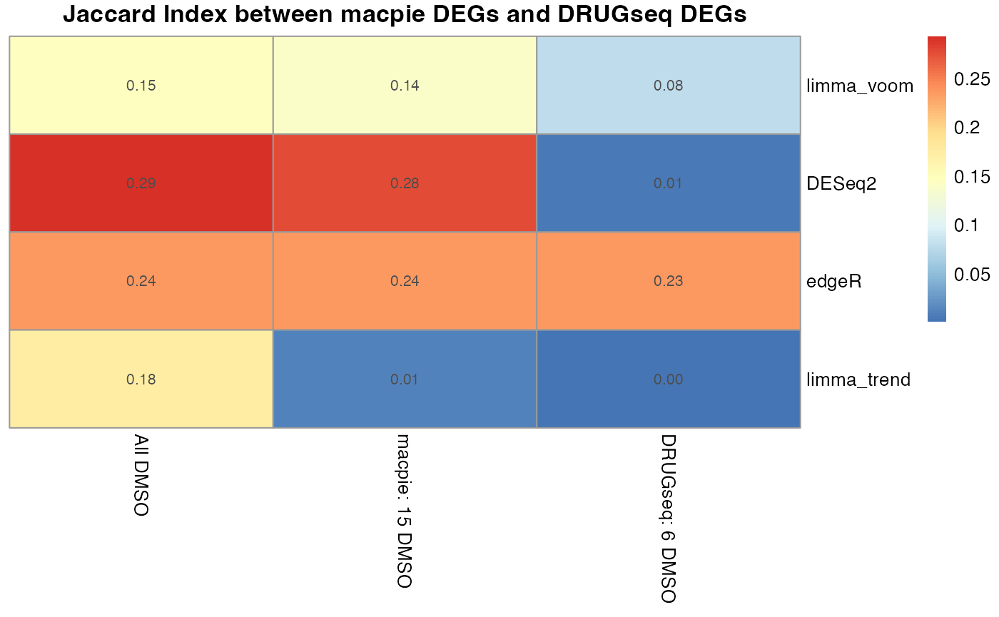

Overlap of DEGs using all DMSO wells

library(UpSetR)
all_dmso <- list(
  limma_voom = methods_res$limma_voom$top_table %>% filter(p_value_adj <0.05 & log2FC>0) %>% select(gene) %>% pull(),
  DESeq2 = methods_res$DESeq2$top_table %>% filter(p_value_adj <0.05 & log2FC>0) %>% select(gene) %>% pull(),
  edgeR = methods_res$edgeR$top_table %>% filter(p_value_adj <0.05 & log2FC>0) %>% select(gene) %>% pull(),
  limma_trend = methods_res$limma_trend$top_table %>% filter(p_value_adj <0.05 & log2FC>0) %>% select(gene) %>% pull(),
  DRUGseq = drugseq_deg
)
upset(fromList(all_dmso), 
      nsets = 5, 
      order.by = "freq",
      main.bar.color = "black",
      sets.bar.color = "gray23",
      text.scale = c(2, 2, 2, 1.5, 2, 1.5),
      mainbar.y.label = "Number of common DEGs",
      sets.x.label = "Number of DEGs")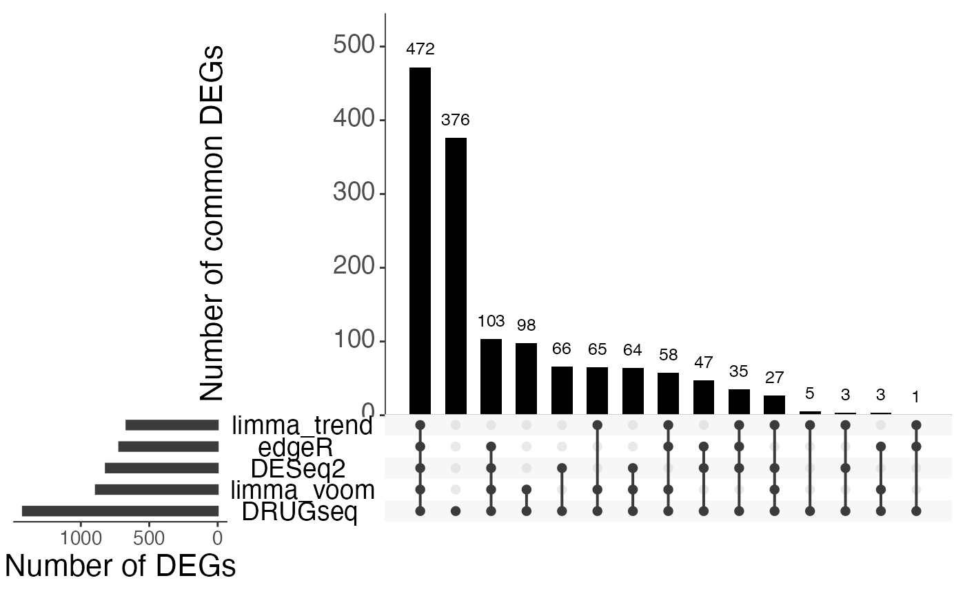

Overlap of DEGs using 15 DMSO wells

five_dmso <- list(
  limma_voom = five_dmso_methods_res$limma_voom$top_table %>% filter(p_value_adj <0.05 & log2FC>0) %>% select(gene) %>% pull(),
  DESeq2 = five_dmso_methods_res$DESeq2$top_table %>% filter(p_value_adj <0.05 & log2FC>0) %>% select(gene) %>% pull(),
  edgeR = five_dmso_methods_res$edgeR$top_table %>% filter(p_value_adj <0.05 & log2FC>0) %>% select(gene) %>% pull(),
  limma_trend = five_dmso_methods_res$limma_trend$top_table %>% filter(p_value_adj <0.05 & log2FC>0) %>% select(gene) %>% pull(),
  DRUGseq = drugseq_deg
)
upset(fromList(five_dmso), 
      nsets = 5, 
      order.by = "freq",
      main.bar.color = "black",
      sets.bar.color = "gray23",
      text.scale = c(2, 2, 2, 1.5, 2, 1.5),
      mainbar.y.label = "Number of common DEGs",
      sets.x.label = "Number of DEGs")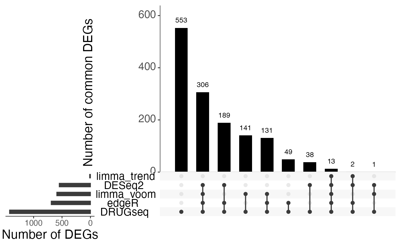

Overlap of DEGs using 6 DMSO wells

robust_dmso <- list(
  limma_voom = robust_dmso_methods_res$limma_voom$top_table %>% filter(p_value_adj <0.05 & log2FC>0) %>% select(gene) %>% pull(),
  DESeq2 = robust_dmso_methods_res$DESeq2$top_table %>% filter(p_value_adj <0.05 & log2FC>0) %>% select(gene) %>% pull(),
  edgeR = robust_dmso_methods_res$edgeR$top_table %>% filter(p_value_adj <0.05 & log2FC>0) %>% select(gene) %>% pull(),
  limma_trend = robust_dmso_methods_res$limma_trend$top_table %>% filter(p_value_adj <0.05 & log2FC>0) %>% select(gene) %>% pull(),
  DRUGseq = drugseq_deg
)
upset(fromList(robust_dmso), 
      nsets = 5, 
      order.by = "freq",
      main.bar.color = "black",
      sets.bar.color = "gray23",
      text.scale = c(2, 2, 2, 1.5, 2, 1.5),
      mainbar.y.label = "Number of common DEGs",
      sets.x.label = "Number of DEGs")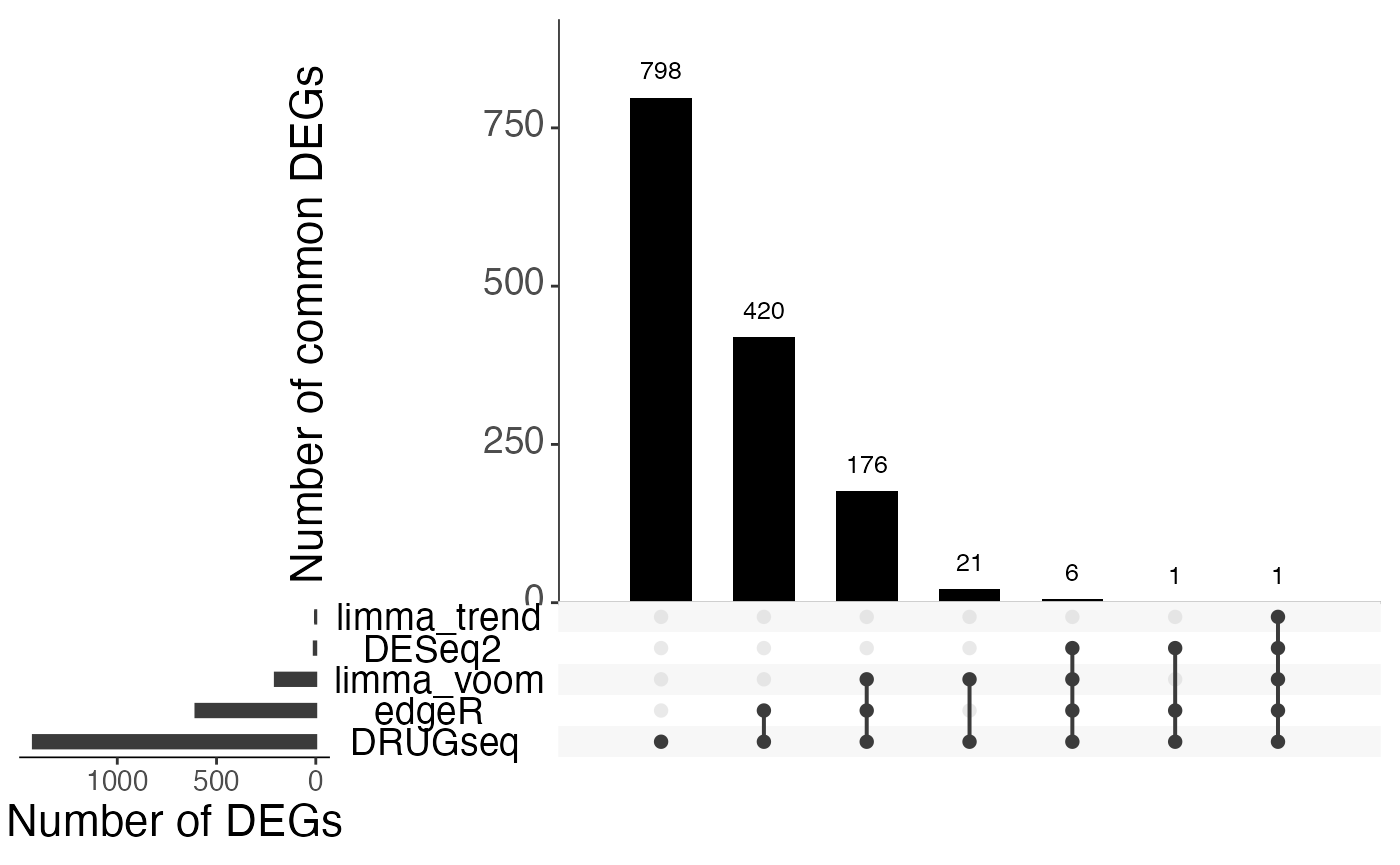

From Jaccard heatmap and UpSet plots, with all 48 DMSO controls, DESeq2 and edgeR show the largest overlaps with DRGseq (Jaccard = 0.29 and 0.24; UpSet intersections in the hundreds). Limma-voom shows moderate similarity (J=0.15), and limma-trend returns a smaller set (J=0.18). Using 15 macpie-selected DMSO reduces totals and overlaps for most methods; DEseq2 and edgeR remains relatively stable (J = 0.28 and 0.24). With only 6 DRUGseq controls, the DEG sets shrink and pair-wise intersection numbers drop. Especially DEseq2 drops down to J=0.01 and limma_voom reduces to J=0.08. While edgeR remains relatively stable with J=0.23. limma-trend run yields very few DEGs under this setting.

Conclusion

Why robust DMSO subsets can reduce concordance with DRUGseq DEGs?

Possible reasons are that with fewer control samples, our group-aware filter (>= 10 counts in at least 3 samples) becomes more stringent, leading to fewer genes being tested in the DE analysis. This reduction in the number of tested genes can impact the identification of DEGs and their overlap with DRUGseq results. Additionally, having fewer control samples can increase variability in the estimates of dispersion, which can affect the statistical power to detect true DEGs. This increased variability may lead to less consistent results across different methods, thereby reducing concordance with DRUGseq DEGs.

Robust DMSO are selected based on their similarity in overall expression profiles, which may slightly shift normalisation and the mean-variance trend when estimating by TMM/TMMwsp.

QC and filtering:

Use group-aware filtering filter_genes_by_expression to retain genes with consistent expression within each treatment.
Examine any batch/unwanted variation, or potential outliers in the data.

Check zero-inflation:

Run check_zeroinflation before and after filtering to ensure that zero-inflation is minimized.
Decision heuristic: for example, if observed zero proportions are significantly higher than expected under NB after filtering, consider using methods that account for zero-inflation.

Pick controls consciously:

Start with all available controls and assess any potential outliers.

Choose a DE method:

If zero-inflation is present, use a method that accounts for it (compute_single_de edgeR with ZINB-WaVE weights).
If zero-inflation is not a concern,
- edgeR (QLFit) and limma-voom (with TMMwsp): both methods are designed to account for gene-specific variability and handle heteroscedasticity effectively.
- limma-trend: remains suitable for uniformly sequenced experiments as it assumes similar library sizes/sequencing depth.
- DESeq2: strong shrinkage & automatic independent filtering.
If batch/unwanted variation,
- include them in the design (~ batch + condition) or adjust with limma’s removeBatchEffect / edgeR design.
- if strong, apply RUVseq (e.g. RUVg with empirical negative controls or RUVs with replicate samples) before DE. Re-compute normalization after RUV and re-fit your DE model.

Introduction

Converting a DRUGseq plate to a macpie object

1. Metadata import and validation

1.1 Convert DRUGseq metadata to macpie metadata format

1.2 Validate DRUGseq metadata

2. Quality control

2.1 Import data

2.2 Visualize plate layout

2.2 Basic QC metrics

2.2.1 Sample grouping

2.2.2 Correction of the batch effect

Coverting multiple DRUGseq plates to a macpie object

1. Metadata import and validation

2. Quality control

2.1 Import data

2.2 Basic QC metrics

2.2.1 Sample grouping with MDS plot

2.2.2 Sample grouping with UMAP

2.2.3 Distribution of UMI counts

2.2.4 Variability among all replicates

2.2.5 Correction of batch effect

3. Differential gene expression

3.1 Single comparison

3.2 Multiple comparisons

4. Pathway enrichment analysis

4.1 Multiple comparisons

Benchmark

Selecting robust DMSO controls

DRUGseq: 6 robust DMSO wells

macpie: select robust DMSO wells

Plate VH02012942

Plate VH02012944

Plate VH02012956

Summary

DEG concordance

DRUGseq DEG results

macpie DEG results with all DMSO wells

Differential gene expression

Summary table

Overlapping volcano plot

macpie DEG results with 15 robust DMSO wells

Differential gene expression

Summary table

Overlapping volcano plot

macpie DEG results with 6 robust DMSO wells from DRUGseq

Differential gene expression

Summary table

Overlapping volcano plot

Summary of DEG concordance

Overlap of DEGs using all DMSO wells

Overlap of DEGs using 15 DMSO wells

Overlap of DEGs using 6 DMSO wells

Conclusion

Why robust DMSO subsets can reduce concordance with DRUGseq DEGs?

Minimal workflow we recommend for macpie DEG analysis