Overview
This vignette demonstrates how to use macpie with Bioconductor-native containers:
Read raw data into a SingleCellExperiment (SCE) class or SummarizedExperiment (SE) class
Perform Bioconductor-native normalization (
scuttle::logNormCounts)Convert SCE to Seurat object via
sce_to_seurat()-
Run minimal
macpiefunctions in this vignette: Full workflow with macpie functions is shown in the main macpie vignette.
suppressPackageStartupMessages({
  library(macpie)
  library(Seurat)
  library(SingleCellExperiment)
  library(SummarizedExperiment)
  library(Matrix)
  library(scuttle)   # Bioconductor-native normalization
  library(dplyr)
  library(tibble)
  library(DropletUtils)
})
1. Metadata import
Metadata is imported using read_metadata(), and
visualized using plot_metadata_heatmap() like in the main
vignette.
# Load metadata
project_metadata <- system.file("extdata/PMMSq033_metadata.csv", package = "macpie")

# Load metadata
metadata <- read_metadata(project_metadata)
plot_metadata_heatmap(metadata)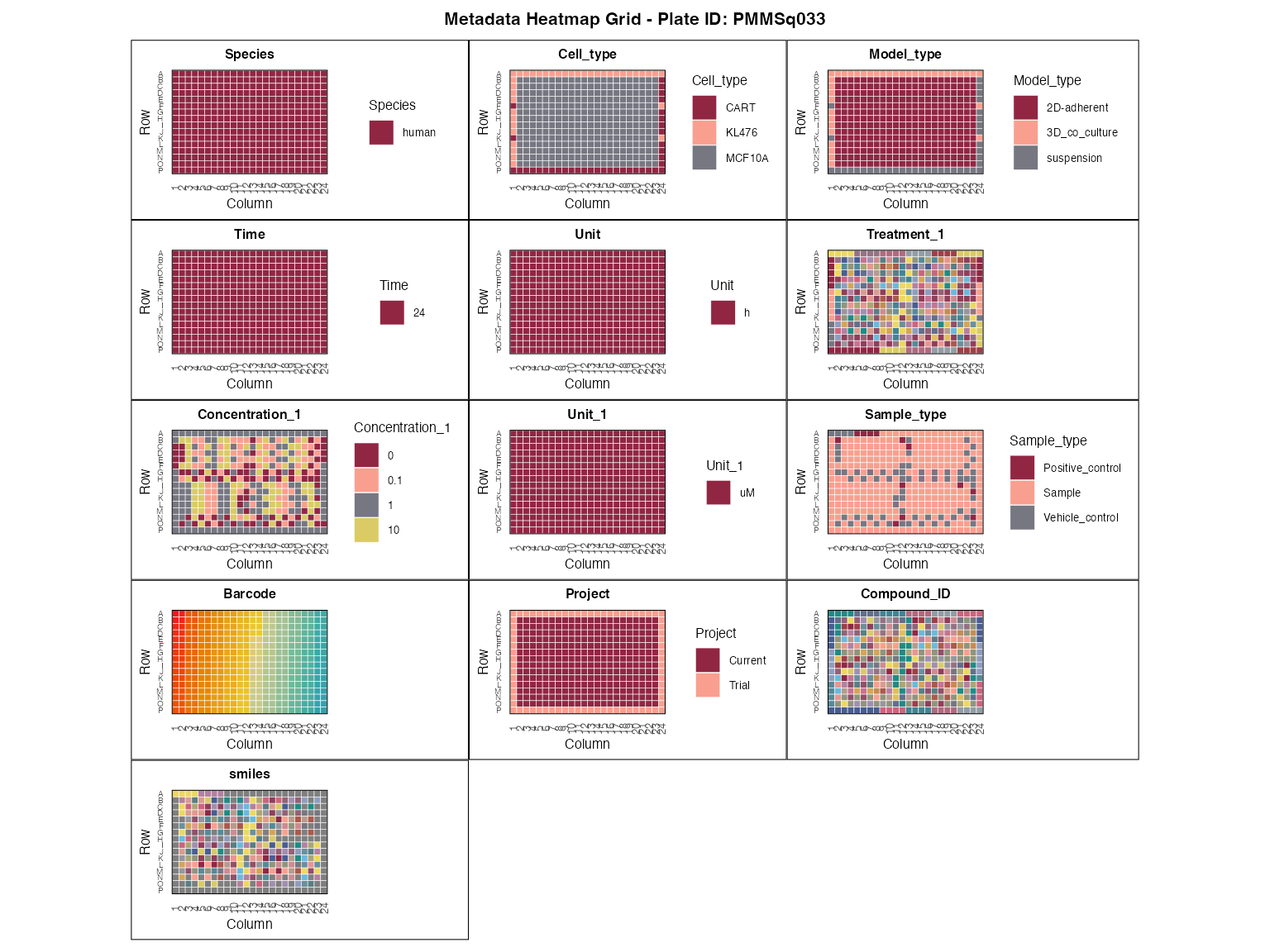
2. Sequencing data import
2.1 Create a SingleCellExperiment object
First, we load raw data into a SingleCellExperiment (SCE) object,
then we add metadata and normalize the data using
scuttle::logNormCounts().
project_rawdata <- paste0(dir, "/macpieData/PMMSq033/raw_matrix")
sce <- read10xCounts(project_rawdata, col.names = TRUE,
                     row.names = "symbol")  # use gene symbols
# add metadata
sce <- SingleCellExperiment(assays = list(counts = counts(sce)))
# with match barcodes
colData(sce) <- DataFrame(metadata[match(colnames(sce), metadata$Barcode), ])


# normalize (adds 'logcounts' assay)
sce <- scuttle::logNormCounts(sce)
2.2 Convert SCE to Seurat object
By default, sce_to_seurat() uses the “counts” assay as
the raw counts and “logcounts” assay as the normalized data. You can
change these parameters if your SCE object has different assay names.
The function also requires the name of the column in the
colData that contains the cell IDs (barcodes). We also
address issues with gene names (e.g., underscores) to ensure
compatibility with Seurat.
to_seurat <- sce_to_seurat(sce,
                          counts = "counts",
                          log_counts = "logcounts",
                          assay = "RNA",
                          cell_id_col = "Barcode",
                          project_name = "PMMSq033")
to_seurat
#> # A Seurat-tibble abstraction: 384 × 22
#> # Features=62700 | Cells=384 | Active assay=RNA | Assays=RNA
#>    .cell      orig.ident nCount_RNA nFeature_RNA Plate_ID Well_ID Row   Column
#>    <chr>      <fct>           <dbl>        <int> <chr>    <chr>   <chr>  <int>
#>  1 AACAAGGTAC PMMSq033          440          348 PMMSq033 A01     A          1
#>  2 AACAATCAGG PMMSq033         6189         3173 PMMSq033 B01     B          1
#>  3 AACACCTAGT PMMSq033          831          590 PMMSq033 A02     A          2
#>  4 AACAGGCAAT PMMSq033         8001         3094 PMMSq033 B02     B          2
#>  5 AACATGGAGA PMMSq033         6998         3307 PMMSq033 C01     C          1
#>  6 AACATTACCG PMMSq033         3494         2004 PMMSq033 D01     D          1
#>  7 AACCAGCCAG PMMSq033        69775        12721 PMMSq033 C02     C          2
#>  8 AACCAGTTGA PMMSq033        52440        11345 PMMSq033 D02     D          2
#>  9 AACCGCGACT PMMSq033         5726         2866 PMMSq033 E01     E          1
#> 10 AACCGGAAGG PMMSq033           63           57 PMMSq033 F01     F          1
#> # ℹ 374 more rows
#> # ℹ 14 more variables: Species <chr>, Cell_type <chr>, Model_type <chr>,
#> #   Time <fct>, Unit <chr>, Treatment_1 <chr>, Concentration_1 <fct>,
#> #   Unit_1 <chr>, Sample_type <chr>, Barcode <chr>, Project <chr>,
#> #   Compound_ID <chr>, smiles <chr>, sizeFactor <dbl>
2.3 Sanity check
This is to check that the conversion was successful and that the data in the Seurat object matches the original SCE object. We should have the same number of wells, and the well barcodes should match. Additionally, the gene names in the Seurat object should match those in the SCE object.
3. Basic quality control and filtering
Now, we can use some basic macpie functions for quality
control and filtering.
to_seurat <- to_seurat %>%
  mutate(combined_id = str_c(Treatment_1, Concentration_1, sep = "_")) %>%
  mutate(combined_id = gsub(" ", "", .data$combined_id)) %>%
  mutate(combined_id = make.names(combined_id))


# Filter by read count per sample group
to_seurat <- filter_genes_by_expression(to_seurat,
                                  group_by = "combined_id",
                                  min_counts = 5,
                                  min_samples = 1)
3.1 Visualize QC metrics
We should expect to see same violin plots as using Seurat object in the main vigette.
to_seurat[["percent.mt"]] <- PercentageFeatureSet(to_seurat, pattern = "^mt-|^MT-")
to_seurat[["percent.ribo"]] <- PercentageFeatureSet(to_seurat, pattern = "^Rp[slp][[:digit:]]|^Rpsa|^RP[SLP][[:digit:]]|^RPSA")

# Example of a function from Seurat quality control
VlnPlot(to_seurat, features = c("nFeature_RNA", "nCount_RNA", "percent.mt", "percent.ribo"),
        ncol = 4, group.by = "Sample_type") &
scale_fill_manual(values = macpie_colours$discrete) 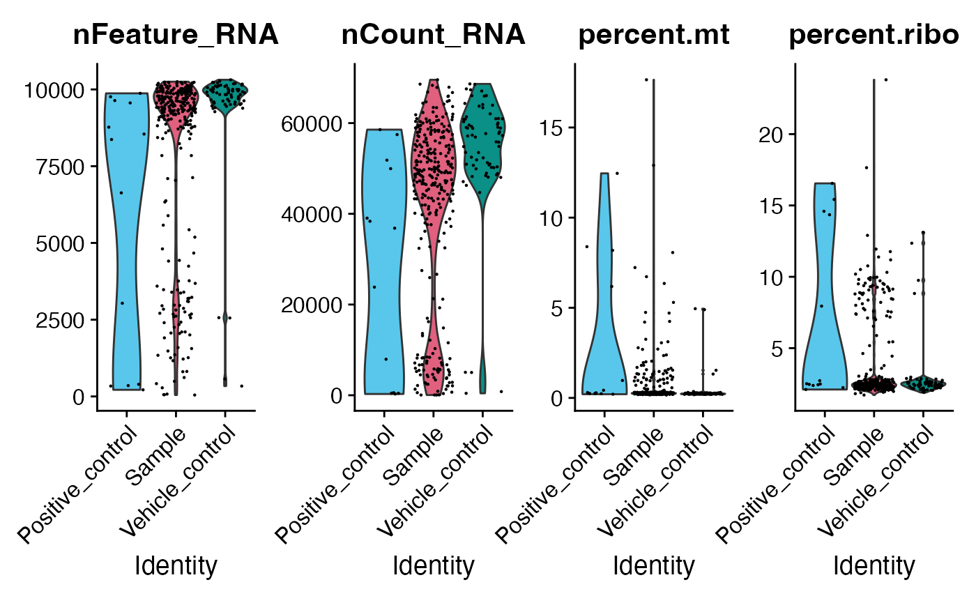
3.2 Subset data for a specific project and visualize plate layout
Here we subset the data to include only cells from the “Current”
project and visualize the plate layout using
plot_plate_layout(). The interactive plot allows us to
hover over wells to see detailed information.
This plot should be identical to the one generated using a Seurat object in the main vignette.
unique(to_seurat$Project)
#> [1] "Trial"   "Current"
to_seurat <- to_seurat %>%
  filter(Project == "Current")

# Interactive QC plot plate layout (all metadata columns can be used):
p <- plot_plate_layout(to_seurat, "nCount_RNA", "combined_id")
girafe(ggobj = p,
  fonts = list(sans = "sans"),
  options = list(
    opts_hover(css = "stroke:black; stroke-width:0.8px;")  # <- slight darkening
  ))
4. Summary
In this vignette, we demonstrated how to work with Bioconductor-native classes using macpie. We covered the following steps:
Importing metadata and visualizing it.
Creating a SingleCellExperiment object from raw data, adding metadata, and normalizing the data.
Converting the SingleCellExperiment object to a Seurat object using
sce_to_seurat().Performing basic quality control and filtering using
macpiefunctions, including visualizing QC metrics and plotting the plate layout.